# Downloading packages -------------------------------------------------------
- Downloading here from CRAN ...                OK [32.2 Kb]
- Downloading rprojroot from CRAN ...           OK [58.5 Kb in 0.17s]
- Downloading tidyverse from CRAN ...           OK [688.1 Kb]
- Downloading broom from CRAN ...               OK [636 Kb]
- Downloading backports from CRAN ...           OK [30 Kb in 0.18s]
- Downloading conflicted from CRAN ...          OK [16.7 Kb]
- Downloading dbplyr from CRAN ...              OK [752.6 Kb]
- Downloading blob from CRAN ...                OK [10.4 Kb]
- Downloading DBI from CRAN ...                 OK [1.1 Mb]
- Downloading dtplyr from CRAN ...              OK [147.4 Kb]
- Downloading data.table from CRAN ...          OK [5.6 Mb in 0.2s]
- Downloading forcats from CRAN ...             OK [287.3 Kb]
- Downloading ggplot2 from CRAN ...             OK [3.4 Mb]
- Downloading gtable from CRAN ...              OK [144.7 Kb]
- Downloading isoband from CRAN ...             OK [1.5 Mb in 0.18s]
- Downloading scales from CRAN ...              OK [321 Kb]
- Downloading farver from CRAN ...              OK [1.2 Mb in 0.14s]
- Downloading labeling from CRAN ...            OK [9.9 Kb in 0.19s]
- Downloading RColorBrewer from CRAN ...        OK [11.4 Kb in 0.18s]
- Downloading viridisLite from CRAN ...         OK [1.2 Mb]
- Downloading googledrive from CRAN ...         OK [1.5 Mb in 0.13s]
- Downloading gargle from CRAN ...              OK [612.9 Kb]
- Downloading httr from CRAN ...                OK [115.7 Kb in 0.12s]
- Downloading curl from CRAN ...                OK [912.2 Kb]
- Downloading openssl from CRAN ...             OK [1.2 Mb in 0.12s]
- Downloading askpass from CRAN ...             OK [5.9 Kb in 0.13s]
- Downloading sys from CRAN ...                 OK [19.5 Kb in 0.13s]
- Downloading uuid from CRAN ...                OK [78.8 Kb]
- Downloading googlesheets4 from CRAN ...       OK [227.1 Kb in 0.18s]
- Downloading ids from CRAN ...                 OK [89.1 Kb]
- Downloading rematch2 from CRAN ...            OK [13.1 Kb]
- Downloading haven from CRAN ...               OK [309.5 Kb in 0.18s]
- Downloading modelr from CRAN ...              OK [118.6 Kb]
- Downloading ragg from CRAN ...                OK [420.7 Kb in 0.13s]
- Downloading systemfonts from CRAN ...         OK [103.5 Kb]
- Downloading textshaping from CRAN ...         OK [74 Kb]
- Downloading reprex from CRAN ...              OK [1 Mb in 0.13s]
- Downloading callr from CRAN ...               OK [101.9 Kb]
- Downloading processx from CRAN ...            OK [161.3 Kb in 0.18s]
- Downloading ps from CRAN ...                  OK [164 Kb in 0.12s]
- Downloading rstudioapi from CRAN ...          OK [115.7 Kb in 0.12s]
- Downloading rvest from CRAN ...               OK [113.2 Kb]
- Downloading selectr from CRAN ...             OK [40.4 Kb]
- Downloading xml2 from CRAN ...                OK [149.3 Kb]
Successfully downloaded 44 packages in 10 seconds.

The following package(s) will be installed:
- askpass       [1.2.1]
- backports     [1.5.0]
- blob          [1.2.4]
- broom         [1.0.8]
- callr         [3.7.6]
- conflicted    [1.2.0]
- curl          [6.3.0]
- data.table    [1.17.6]
- DBI           [1.2.3]
- dbplyr        [2.5.0]
- dtplyr        [1.3.1]
- farver        [2.1.2]
- forcats       [1.0.0]
- gargle        [1.5.2]
- ggplot2       [3.5.2]
- googledrive   [2.1.1]
- googlesheets4 [1.1.1]
- gtable        [0.3.6]
- haven         [2.5.5]
- here          [1.0.1]
- httr          [1.4.7]
- ids           [1.0.1]
- isoband       [0.2.7]
- labeling      [0.4.3]
- modelr        [0.1.11]
- openssl       [2.3.3]
- processx      [3.8.6]
- ps            [1.9.1]
- ragg          [1.4.0]
- RColorBrewer  [1.1-3]
- rematch2      [2.1.2]
- reprex        [2.1.1]
- rprojroot     [2.0.4]
- rstudioapi    [0.17.1]
- rvest         [1.0.4]
- scales        [1.4.0]
- selectr       [0.4-2]
- sys           [3.4.3]
- systemfonts   [1.2.3]
- textshaping   [1.0.1]
- tidyverse     [2.0.0]
- uuid          [1.2-1]
- viridisLite   [0.4.2]
- xml2          [1.3.8]
These packages will be installed into "~/work/notebook/notebook/renv/library/linux-ubuntu-noble/R-4.4/x86_64-pc-linux-gnu".

# Installing packages --------------------------------------------------------
- Installing rprojroot ...                      OK [built from source and cached in 1.3s]
- Installing here ...                           OK [built from source and cached in 1.1s]
- Installing backports ...                      OK [built from source and cached in 1.6s]
- Installing broom ...                          OK [built from source and cached in 6.1s]
- Installing conflicted ...                     OK [built from source and cached in 1.5s]
- Installing blob ...                           OK [built from source and cached in 1.6s]
- Installing DBI ...                            OK [built from source and cached in 3.5s]
- Installing dbplyr ...                         OK [built from source and cached in 11s]
- Installing data.table ...                     OK [built from source and cached in 19s]
- Installing dtplyr ...                         OK [built from source and cached in 3.6s]
- Installing forcats ...                        OK [built from source and cached in 2.0s]
- Installing gtable ...                         OK [built from source and cached in 1.9s]
- Installing isoband ...                        OK [built from source and cached in 4.4s]
- Installing farver ...                         OK [built from source and cached in 18s]
- Installing labeling ...                       OK [built from source and cached in 1.3s]
- Installing RColorBrewer ...                   OK [built from source and cached in 1.4s]
- Installing viridisLite ...                    OK [built from source and cached in 1.1s]
- Installing scales ...                         OK [built from source and cached in 4.6s]
- Installing ggplot2 ...                        OK [built from source and cached in 14s]
- Installing curl ...                           OK [built from source and cached in 3.6s]
- Installing sys ...                            OK [built from source and cached in 1.3s]
- Installing askpass ...                        OK [built from source and cached in 1.1s]
- Installing openssl ...                        OK [built from source and cached in 5.2s]
- Installing httr ...                           OK [built from source and cached in 3.1s]
- Installing gargle ...                         OK [built from source and cached in 3.8s]
- Installing uuid ...                           OK [built from source and cached in 3.9s]
- Installing googledrive ...                    OK [built from source and cached in 3.5s]
- Installing ids ...                            OK [built from source and cached in 1.2s]
- Installing rematch2 ...                       OK [built from source and cached in 1.9s]
- Installing googlesheets4 ...                  OK [built from source and cached in 3.7s]
- Installing haven ...                          OK [built from source and cached in 14s]
- Installing modelr ...                         OK [built from source and cached in 2.5s]
- Installing systemfonts ...                    OK [built from source and cached in 21s]
- Installing textshaping ...                    OK [built from source and cached in 12s]
- Installing ragg ...                           OK [built from source and cached in 1.9m]
- Installing ps ...                             OK [built from source and cached in 4.6s]
- Installing processx ...                       OK [built from source and cached in 4.1s]
- Installing callr ...                          OK [built from source and cached in 3.4s]
- Installing rstudioapi ...                     OK [built from source and cached in 1.6s]
- Installing reprex ...                         OK [built from source and cached in 2.0s]
- Installing selectr ...                        OK [built from source and cached in 5.9s]
- Installing xml2 ...                           OK [built from source and cached in 6.4s]
- Installing rvest ...                          OK [built from source and cached in 2.7s]
- Installing tidyverse ...                      OK [built from source and cached in 2.8s]
Successfully installed 44 packages in 5.5 minutes.
R
R Packages
An R package usually includes:
- reusable functions
- documentation describing how to use the function
- sample data
Primitive Data Types
The primitive (also known as singleton/simple) data types in R are:
- character
- numeric
- logical
- raw
- imaginary numbers
To know the datatype of an object, run the command:
To know the type of the variables of each variable.
Mixing Data Types
- character + numeric –> character
- numeric + logical –> numeric
- numeric + character + logical –> character
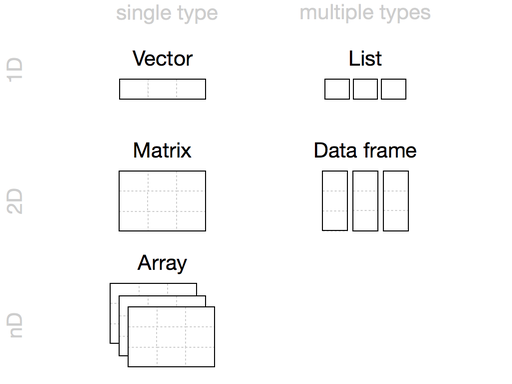
Compound Data Types
The compound (also know as collection/sttructure) data types in R are:
- vector: hold single type of data
Creating Vector
The c() function (combine multiple elements) can be used to create vectors in R.
x <- c(1, 2, 3, 4)- matrix: 2D vector
- array: nD vector
- list: generic vector, can hold mixed type of data, eg, one element can be a character, another can be a list of integers, and the third could be a logical
- data frame: table where columns represent vectors
- tibbles: data frames, but slightly tweaked to work better with
tidyverse–when printing tibbles, only the first few columns that fit into the screen will be shown
Printing tibble All Columns
To construct small tibble by hand, use the tribble function as follows:
- factor
To know the data structure and length of the object, run the command:
Basics Operations
Assignment
[1] 3Getting Help
Dealing with Structure
# concatenate set of values to create vector
weight_g <- c(50, 60, 3, 9)
animals <- c("dog", "bat", "cat")

# utilizing logical values to pull specific values
weight_g[weight_g < 10 & weight_g > 60 | weight_g == 50]
[1] 50[1] "dog" "cat"[1] "dog" "cat"Statistics
Initial Steps
File Paths
The here package makes it easy to point to files starting from the project main directory.
Store Locally
Loading file from repository and saving it locally on disk. It is always a good idea to structure the workspace–for more information, see Best Practices for Scientific Computing paper.
Load Locally
Rows: 34,786
Columns: 13
$ record_id       <int> 1, 72, 224, 266, 349, 363, 435, 506, 588, 661, 748, 84…
$ month           <int> 7, 8, 9, 10, 11, 11, 12, 1, 2, 3, 4, 5, 6, 8, 9, 10, 1…
$ day             <int> 16, 19, 13, 16, 12, 12, 10, 8, 18, 11, 8, 6, 9, 5, 4, …
$ year            <int> 1977, 1977, 1977, 1977, 1977, 1977, 1977, 1978, 1978, …
$ plot_id         <int> 2, 2, 2, 2, 2, 2, 2, 2, 2, 2, 2, 2, 2, 2, 2, 2, 2, 2, …
$ species_id      <chr> "NL", "NL", "NL", "NL", "NL", "NL", "NL", "NL", "NL", …
$ sex             <chr> "M", "M", "", "", "", "", "", "", "M", "", "", "M", "M…
$ hindfoot_length <int> 32, 31, NA, NA, NA, NA, NA, NA, NA, NA, NA, 32, NA, 34…
$ weight          <int> NA, NA, NA, NA, NA, NA, NA, NA, 218, NA, NA, 204, 200,…
$ genus           <chr> "Neotoma", "Neotoma", "Neotoma", "Neotoma", "Neotoma",…
$ species         <chr> "albigula", "albigula", "albigula", "albigula", "albig…
$ taxa            <chr> "Rodent", "Rodent", "Rodent", "Rodent", "Rodent", "Rod…
$ plot_type       <chr> "Control", "Control", "Control", "Control", "Control",…
Clean Names
Inspecting Data
'data.frame':   34786 obs. of  13 variables:
 $ record_id      : int  1 72 224 266 349 363 435 506 588 661 ...
 $ month          : int  7 8 9 10 11 11 12 1 2 3 ...
 $ day            : int  16 19 13 16 12 12 10 8 18 11 ...
 $ year           : int  1977 1977 1977 1977 1977 1977 1977 1978 1978 1978 ...
 $ plot_id        : int  2 2 2 2 2 2 2 2 2 2 ...
 $ species_id     : chr  "NL" "NL" "NL" "NL" ...
 $ sex            : chr  "M" "M" "" "" ...
 $ hindfoot_length: int  32 31 NA NA NA NA NA NA NA NA ...
 $ weight         : int  NA NA NA NA NA NA NA NA 218 NA ...
 $ genus          : chr  "Neotoma" "Neotoma" "Neotoma" "Neotoma" ...
 $ species        : chr  "albigula" "albigula" "albigula" "albigula" ...
 $ taxa           : chr  "Rodent" "Rodent" "Rodent" "Rodent" ...
$ plot_type : chr "Control" "Control" "Control" "Control" ...Rows: 0
Columns: 13
$ record_id <int>
$ month <int>
$ day <int>
$ year <int>
$ plot_id <int>
$ species_id <chr>
$ sex <chr>
$ hindfoot_length <int>
$ weight <int>
$ genus <chr>
$ species <chr>
$ taxa <chr>
$ plot_type <chr> record_id month day year plot_id
Min. : 1 Min. : 1.000 Min. : 1.0 Min. :1977 Min. : 1.00
1st Qu.: 8964 1st Qu.: 4.000 1st Qu.: 9.0 1st Qu.:1984 1st Qu.: 5.00
Median :17762 Median : 6.000 Median :16.0 Median :1990 Median :11.00
Mean :17804 Mean : 6.474 Mean :16.1 Mean :1990 Mean :11.34
3rd Qu.:26655 3rd Qu.:10.000 3rd Qu.:23.0 3rd Qu.:1997 3rd Qu.:17.00
Max. :35548 Max. :12.000 Max. :31.0 Max. :2002 Max. :24.00
species_id sex hindfoot_length weight
Length:34786 Length:34786 Min. : 2.00 Min. : 4.00
Class :character Class :character 1st Qu.:21.00 1st Qu.: 20.00
Mode :character Mode :character Median :32.00 Median : 37.00
Mean :29.29 Mean : 42.67
3rd Qu.:36.00 3rd Qu.: 48.00
Max. :70.00 Max. :280.00
NA's :3348 NA's :2503
genus species taxa plot_type
Length:34786 Length:34786 Length:34786 Length:34786
Class :character Class :character Class :character Class :character
Mode :character Mode :character Mode :character Mode :character
Print top and bottom obervations
  record_id month day year plot_id species_id sex hindfoot_length weight
1         1     7  16 1977       2         NL   M              32     NA
2        72     8  19 1977       2         NL   M              31     NA
3       224     9  13 1977       2         NL                  NA     NA
4       266    10  16 1977       2         NL                  NA     NA
5       349    11  12 1977       2         NL                  NA     NA
6       363    11  12 1977       2         NL                  NA     NA
    genus  species   taxa plot_type
1 Neotoma albigula Rodent   Control
2 Neotoma albigula Rodent   Control
3 Neotoma albigula Rodent   Control
4 Neotoma albigula Rodent   Control
5 Neotoma albigula Rodent   Control
6 Neotoma albigula Rodent Control record_id month day year plot_id species_id sex hindfoot_length weight
34781 26787 9 27 1997 7 PL F 21 16
34782 26966 10 25 1997 7 PL M 20 16
34783 27185 11 22 1997 7 PL F 21 22
34784 27792 5 2 1998 7 PL F 20 8
34785 28806 11 21 1998 7 PX NA NA
34786 30986 7 1 2000 7 PX NA NA
genus species taxa plot_type
34781 Peromyscus leucopus Rodent Rodent Exclosure
34782 Peromyscus leucopus Rodent Rodent Exclosure
34783 Peromyscus leucopus Rodent Rodent Exclosure
34784 Peromyscus leucopus Rodent Rodent Exclosure
34785 Chaetodipus sp. Rodent Rodent Exclosure
34786 Chaetodipus sp. Rodent Rodent ExclosureRetrieve specific element/row/column
[1] 1 record_id month day year plot_id species_id sex hindfoot_length weight
1 1 7 16 1977 2 NL M 32 NA
genus species taxa plot_type
1 Neotoma albigula Rodent Control[1] 1 72 224 266 349 363[1] "M" "M" "" "" "" "" Dealing with Factor (Categorical) Columns
R convert columns that contain characters to factors by default. Factors are treated as integer vectors. By default, R sorts levels in alphabetical order.
Reorder factors (to get better plots)
Basic Plotting
Histogram
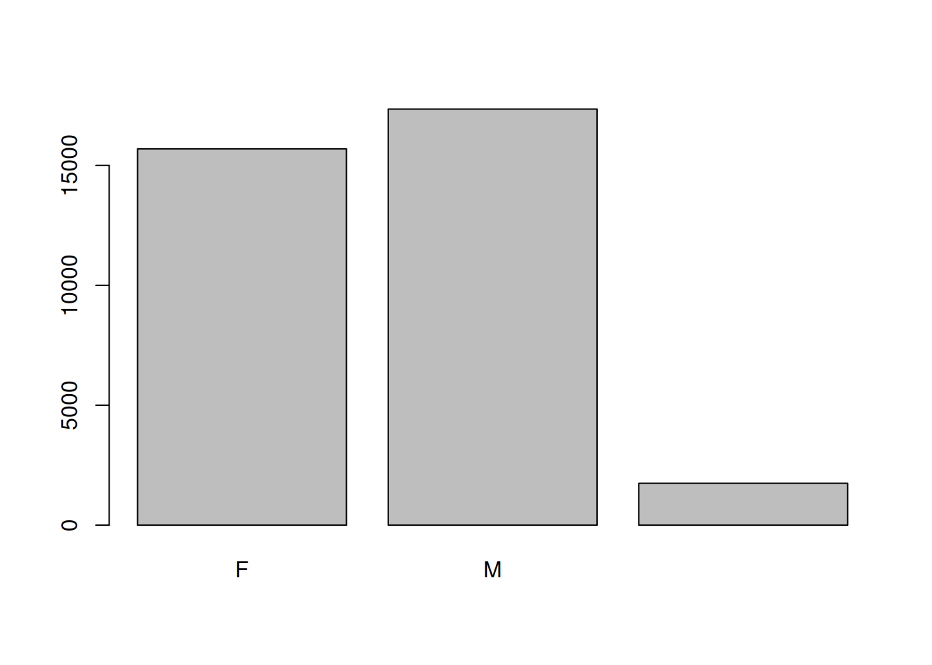
Enhance the plot

Data Manipulation
tdlyr- makes manipulation of data easier
- built to work with data frames directly
- can directly work with data stored in an external database which give the advantage of only bringing what we need to the memory to work on without having to bring the whole database
tidyr- allows to swiftly convert b/w different data formats for plotting & analysis in order to accommodate the different requirements by different functions
- sometime we want one row per measurement
- other times we want the data aggregated like when plotting
- allows to swiftly convert b/w different data formats for plotting & analysis in order to accommodate the different requirements by different functions
Before using tdlyr and tidyr:
- Install
tidyversepackage: umbrella-package that install several packages (tidyr, dplyr, ggplot2 tibble, magrittr, etc.) - Load the package each session
Load packages
Load & inspect data
# notice the '_' instead of '.' of basic R
surveys <- read_csv(here("data", "portal_data_joined.csv"))

str(surveys) # structure: tbl_df (tibble)
spc_tbl_ [34,786 × 13] (S3: spec_tbl_df/tbl_df/tbl/data.frame)
$ record_id : num [1:34786] 1 72 224 266 349 363 435 506 588 661 ...
$ month : num [1:34786] 7 8 9 10 11 11 12 1 2 3 ...
$ day : num [1:34786] 16 19 13 16 12 12 10 8 18 11 ...
$ year : num [1:34786] 1977 1977 1977 1977 1977 ...
$ plot_id : num [1:34786] 2 2 2 2 2 2 2 2 2 2 ...
$ species_id : chr [1:34786] "NL" "NL" "NL" "NL" ...
$ sex : chr [1:34786] "M" "M" NA NA ...
$ hindfoot_length: num [1:34786] 32 31 NA NA NA NA NA NA NA NA ...
$ weight : num [1:34786] NA NA NA NA NA NA NA NA 218 NA ...
$ genus : chr [1:34786] "Neotoma" "Neotoma" "Neotoma" "Neotoma" ...
$ species : chr [1:34786] "albigula" "albigula" "albigula" "albigula" ...
$ taxa : chr [1:34786] "Rodent" "Rodent" "Rodent" "Rodent" ...
$ plot_type : chr [1:34786] "Control" "Control" "Control" "Control" ...
- attr(*, "spec")=
.. cols(
.. record_id = col_double(),
.. month = col_double(),
.. day = col_double(),
.. year = col_double(),
.. plot_id = col_double(),
.. species_id = col_character(),
.. sex = col_character(),
.. hindfoot_length = col_double(),
.. weight = col_double(),
.. genus = col_character(),
.. species = col_character(),
.. taxa = col_character(),
.. plot_type = col_character()
.. )
- attr(*, "problems")=<externalptr> Selection
Select certain columns
# A tibble: 34,786 × 3
   plot_id species_id weight
     <dbl> <chr>       <dbl>
 1       2 NL             NA
 2       2 NL             NA
 3       2 NL             NA
 4       2 NL             NA
 5       2 NL             NA
 6       2 NL             NA
 7       2 NL             NA
 8       2 NL             NA
 9       2 NL            218
10       2 NL             NA
# ℹ 34,776 more rows
Select all columns except …
# A tibble: 34,786 × 12
   record_id month   day  year plot_id species_id hindfoot_length weight genus
       <dbl> <dbl> <dbl> <dbl>   <dbl> <chr>                <dbl>  <dbl> <chr>
 1         1     7    16  1977       2 NL                      32     NA Neotoma
 2        72     8    19  1977       2 NL                      31     NA Neotoma
 3       224     9    13  1977       2 NL                      NA     NA Neotoma
 4       266    10    16  1977       2 NL                      NA     NA Neotoma
 5       349    11    12  1977       2 NL                      NA     NA Neotoma
 6       363    11    12  1977       2 NL                      NA     NA Neotoma
 7       435    12    10  1977       2 NL                      NA     NA Neotoma
 8       506     1     8  1978       2 NL                      NA     NA Neotoma
 9       588     2    18  1978       2 NL                      NA    218 Neotoma
10       661     3    11  1978       2 NL                      NA     NA Neotoma
# ℹ 34,776 more rows
# ℹ 3 more variables: species <chr>, taxa <chr>, plot_type <chr>
Select rows based on criteria
# A tibble: 1,180 × 13
   record_id month   day  year plot_id species_id sex   hindfoot_length weight
       <dbl> <dbl> <dbl> <dbl>   <dbl> <chr>      <chr>           <dbl>  <dbl>
 1     22314     6     7  1995       2 NL         M                  34     NA
 2     22728     9    23  1995       2 NL         F                  32    165
 3     22899    10    28  1995       2 NL         F                  32    171
 4     23032    12     2  1995       2 NL         F                  33     NA
 5     22003     1    11  1995       2 DM         M                  37     41
 6     22042     2     4  1995       2 DM         F                  36     45
 7     22044     2     4  1995       2 DM         M                  37     46
 8     22105     3     4  1995       2 DM         F                  37     49
 9     22109     3     4  1995       2 DM         M                  37     46
10     22168     4     1  1995       2 DM         M                  36     48
# ℹ 1,170 more rows
# ℹ 4 more variables: genus <chr>, species <chr>, taxa <chr>, plot_type <chr>
Piping
Sending the results of one function to another
# in multiple steps
survey_less5 <- filter(surveys, weight < 5)
survey_sml <- select(survey_less5, species_id, sex, weight)

# in one long step
survey_sml <- select(filter(surveys, weight < 5), species_id, sex, weight)

# using pipe %>% of magritter package.  Use Ctrl + Shift + M to add
survey_sml <- surveys %>%
  filter(weight < 5) %>%
  select(species_id, sex, weight)
Summary
Summary of groups (1+ columns)
one factor
# A tibble: 3 × 2
  sex   mean_weight
  <chr>       <dbl>
1 F            42.2
2 M            43.0
3 <NA>         64.7
two factors
# A tibble: 81 × 3
# Groups:   sex [3]
   sex   species     mean_weight
   <chr> <chr>             <dbl>
 1 F     albigula         154.
 2 F     baileyi           30.2
 3 F     eremicus          22.8
 4 F     flavus             7.97
 5 F     fulvescens        13.7
 6 F     fulviventer       69
 7 F     hispidus          69.0
 8 F     leucogaster       31.1
 9 F     leucopus          19.3
10 F     maniculatus       22.1
# ℹ 71 more rows# A tibble: 81 × 3
# Groups: species [40]
species sex mean_weight
<chr> <chr> <dbl>
1 albigula F 154.
2 albigula M 166.
3 albigula <NA> 168.
4 audubonii <NA> NaN
5 baileyi F 30.2
6 baileyi M 33.8
7 baileyi <NA> 30.6
8 bilineata <NA> NaN
9 brunneicapillus <NA> NaN
10 chlorurus <NA> NaN
# ℹ 71 more rowsto avoid using na.rm = FALSE each statistics
surveys %>%
  filter(!is.na(weight)) %>%
  group_by(species, sex) %>%
  summarise(mean_weight = mean(weight), sd_weight = sd(weight), sd_count = n())
# A tibble: 59 × 5
# Groups: species [22]
species sex mean_weight sd_weight sd_count
<chr> <chr> <dbl> <dbl> <int>
1 albigula F 154. 39.2 652
2 albigula M 166. 49.0 484
3 albigula <NA> 168. 44.2 16
4 baileyi F 30.2 5.27 1617
5 baileyi M 33.8 8.27 1188
6 baileyi <NA> 30.6 9.96 5
7 eremicus F 22.8 4.57 568
8 eremicus M 20.6 3.49 689
9 eremicus <NA> 17.7 0.577 3
10 flavus F 7.97 1.69 742
# ℹ 49 more rowsarrange by mean weight
surveys %>%
  filter(!is.na(weight)) %>%
  group_by(species, sex) %>%
  summarise(mean_weight = mean(weight), sd_weight = sd(weight), sd_count = n()) %>%
  arrange(mean_weight)
# A tibble: 59 × 5
# Groups: species [22]
species sex mean_weight sd_weight sd_count
<chr> <chr> <dbl> <dbl> <int>
1 flavus <NA> 6 1.63 4
2 taylori M 7.36 0.842 14
3 flavus M 7.89 1.59 802
4 flavus F 7.97 1.69 742
5 taylori F 9.16 2.24 31
6 montanus M 9.5 1.29 4
7 megalotis M 10.1 1.73 1339
8 montanus F 11 2.16 4
9 megalotis <NA> 11.1 2.57 12
10 megalotis F 11.1 2.56 1184
# ℹ 49 more rowsin descending order
surveys %>%
  filter(!is.na(weight)) %>%
  group_by(species, sex) %>%
  summarise(mean_weight = mean(weight), sd_weight = sd(weight), sd_count = n()) %>%
  arrange(desc(mean_weight))
# A tibble: 59 × 5
# Groups: species [22]
species sex mean_weight sd_weight sd_count
<chr> <chr> <dbl> <dbl> <int>
1 albigula <NA> 168. 44.2 16
2 albigula M 166. 49.0 484
3 albigula F 154. 39.2 652
4 hispidus <NA> 130 NA 1
5 spilosoma M 130 NA 1
6 spectabilis M 122. 24.0 1220
7 spectabilis <NA> 120 18.5 18
8 spectabilis F 118. 21.5 1106
9 fulviventer F 69 37.8 16
10 hispidus F 69.0 29.7 98
# ℹ 49 more rowsby count
surveys %>%
  filter(!is.na(weight)) %>%
  group_by(species, sex) %>%
  summarise(mean_weight = mean(weight), sd_weight = sd(weight), sd_count = n()) %>%
  arrange(sd_count)
# A tibble: 59 × 5
# Groups: species [22]
species sex mean_weight sd_weight sd_count
<chr> <chr> <dbl> <dbl> <int>
1 hispidus <NA> 130 NA 1
2 intermedius <NA> 18 NA 1
3 leucopus <NA> 25 NA 1
4 spilosoma F 57 NA 1
5 spilosoma M 130 NA 1
6 fulviventer <NA> 40.5 6.36 2
7 leucogaster <NA> 29 11.3 2
8 eremicus <NA> 17.7 0.577 3
9 ordii <NA> 50.7 6.51 3
10 sp. F 20.7 1.15 3
# ℹ 49 more rowsCount
Count of a categorical column
Reshaping
Using gather & spreed
prepare the needed data first
creating a 2D table where each dimension represent a category the cell will represent a statistics
tibble [24 × 11] (S3: tbl_df/tbl/data.frame)
 $ plot_id        : num [1:24] 1 2 3 4 5 6 7 8 9 10 ...
 $ Baiomys        : num [1:24] 7 6 8.61 NA 7.75 ...
 $ Chaetodipus    : num [1:24] 22.2 25.1 24.6 23 18 ...
 $ Dipodomys      : num [1:24] 60.2 55.7 52 57.5 51.1 ...
 $ Neotoma        : num [1:24] 156 169 158 164 190 ...
 $ Onychomys      : num [1:24] 27.7 26.9 26 28.1 27 ...
 $ Perognathus    : num [1:24] 9.62 6.95 7.51 7.82 8.66 ...
 $ Peromyscus     : num [1:24] 22.2 22.3 21.4 22.6 21.2 ...
 $ Reithrodontomys: num [1:24] 11.4 10.7 10.5 10.3 11.2 ...
 $ Sigmodon       : num [1:24] NA 70.9 65.6 82 82.7 ...
$ Spermophilus : num [1:24] NA NA NA NA NA NA NA NA NA NA ...# A tibble: 6 × 11
plot_id Baiomys Chaetodipus Dipodomys Neotoma Onychomys Perognathus Peromyscus
<dbl> <dbl> <dbl> <dbl> <dbl> <dbl> <dbl> <dbl>
1 1 7 22.2 60.2 156. 27.7 9.62 22.2
2 2 6 25.1 55.7 169. 26.9 6.95 22.3
3 3 8.61 24.6 52.0 158. 26.0 7.51 21.4
4 4 NA 23.0 57.5 164. 28.1 7.82 22.6
5 5 7.75 18.0 51.1 190. 27.0 8.66 21.2
6 6 NA 24.9 58.6 180. 25.9 7.81 21.8
# ℹ 3 more variables: Reithrodontomys <dbl>, Sigmodon <dbl>, Spermophilus <dbl>bring spread back
tibble [240 × 3] (S3: tbl_df/tbl/data.frame)
 $ plot_id    : num [1:240] 1 2 3 4 5 6 7 8 9 10 ...
 $ genus      : chr [1:240] "Baiomys" "Baiomys" "Baiomys" "Baiomys" ...
$ mean_weight: num [1:240] 7 6 8.61 NA 7.75 ...# A tibble: 6 × 3
plot_id genus mean_weight
<dbl> <chr> <dbl>
1 1 Baiomys 7
2 2 Baiomys 6
3 3 Baiomys 8.61
4 4 Baiomys NA
5 5 Baiomys 7.75
6 6 Baiomys NA Filtering
Remove missing data
Filter those that has sample greater than 50
filter only those in the indicated category
Saving to disk
Visualization
- Help in making complex plots from data frames in simple steps
- ggplot graphics are built step by step by adding new elements; this makes it flexible as well as customization
- To get list of ggplot2 geometric objects:
help.search("gemo_", package="ggplot2") - To know the aesthetic specification each geom_ can take:
vignette("ggplot2-specs")
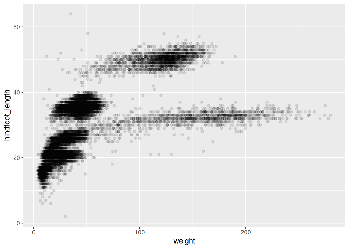
Step 1: Bind the plot to specific data frame
surveys_plot <- ggplot(
  data = survey_complete,
  mapping = aes(x = weight, y = hindfoot_length)
)
surveys_plot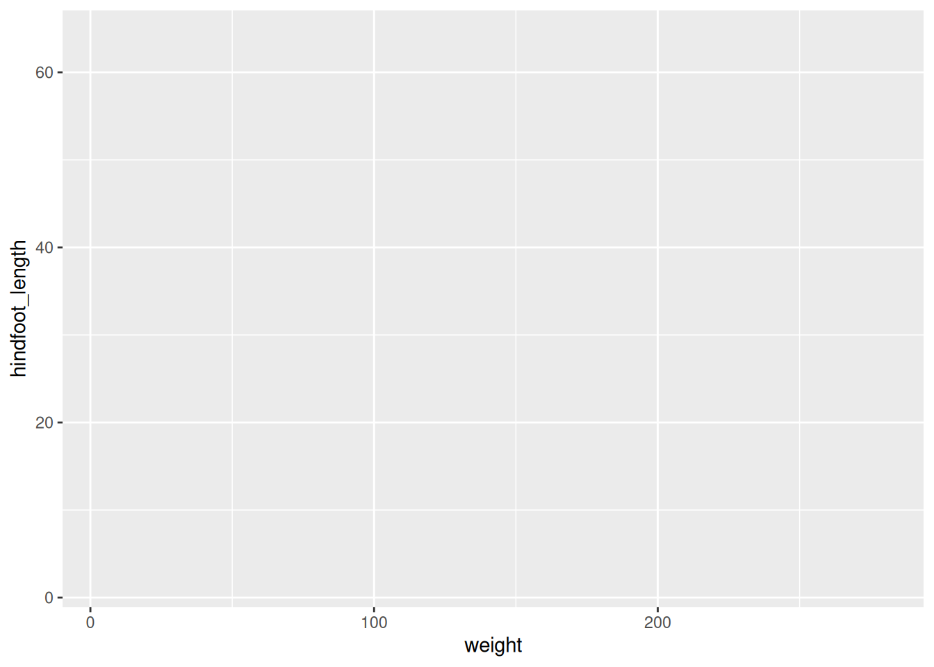
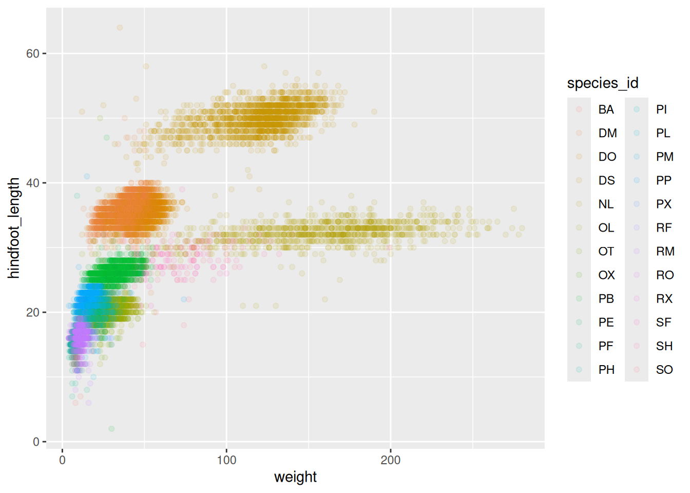
# Color for each group
surveys_plot <- ggplot(
  data = survey_complete,
  mapping = aes(x = weight, y = hindfoot_length),
  color = species_id
)
surveys_plot
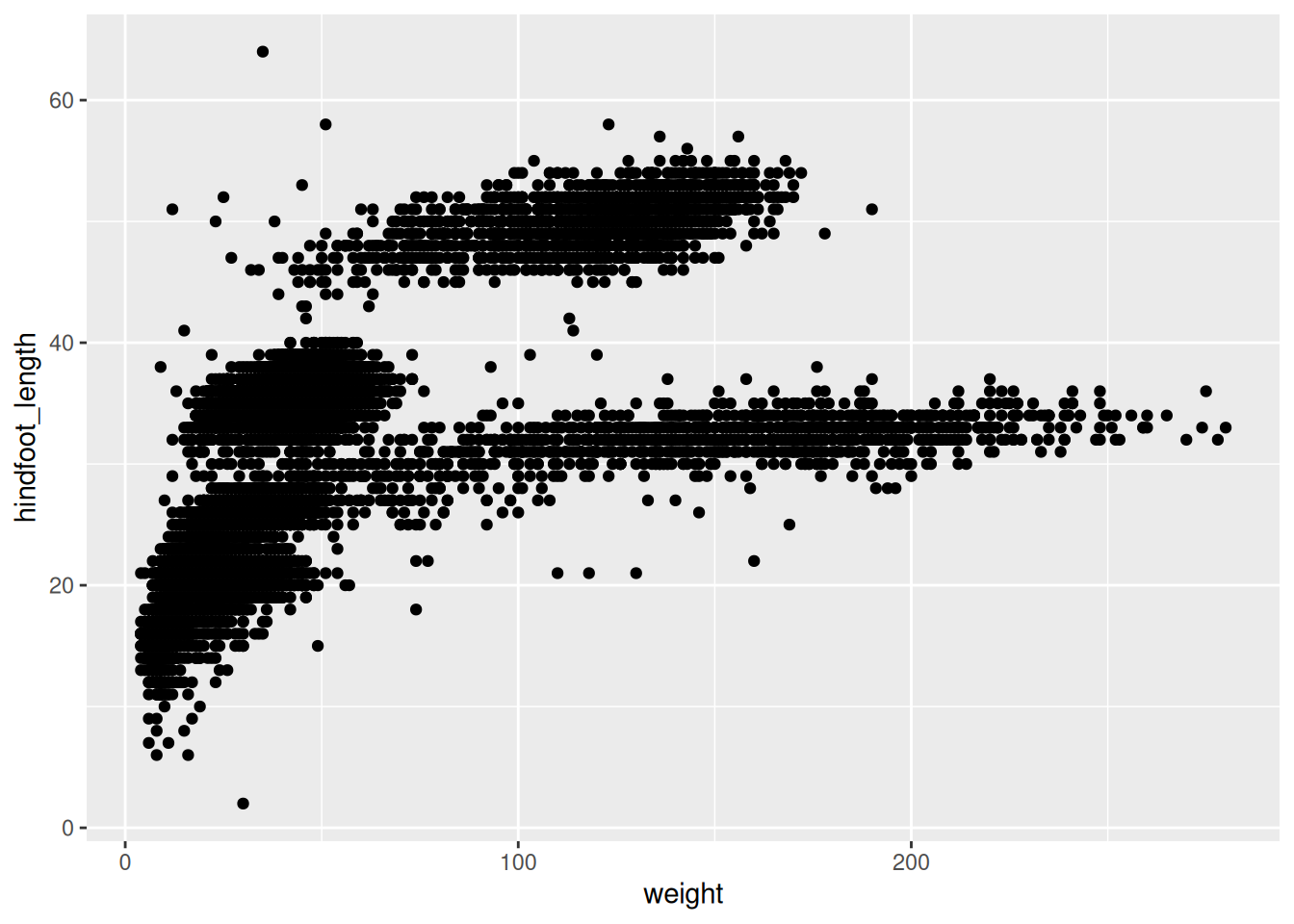
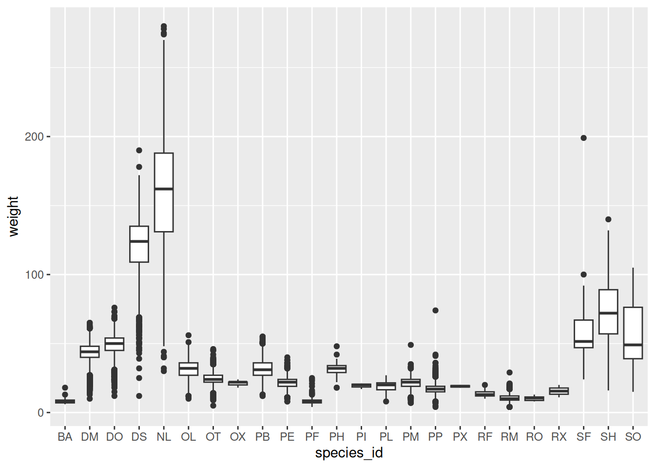
Step 2: Select the type of the plot
- scatter plot, dot plots, etc. > geom_point()
- boxplots > geom_boxplot()
- trend lines, time series, etc. > geom_line()
Scatter plot


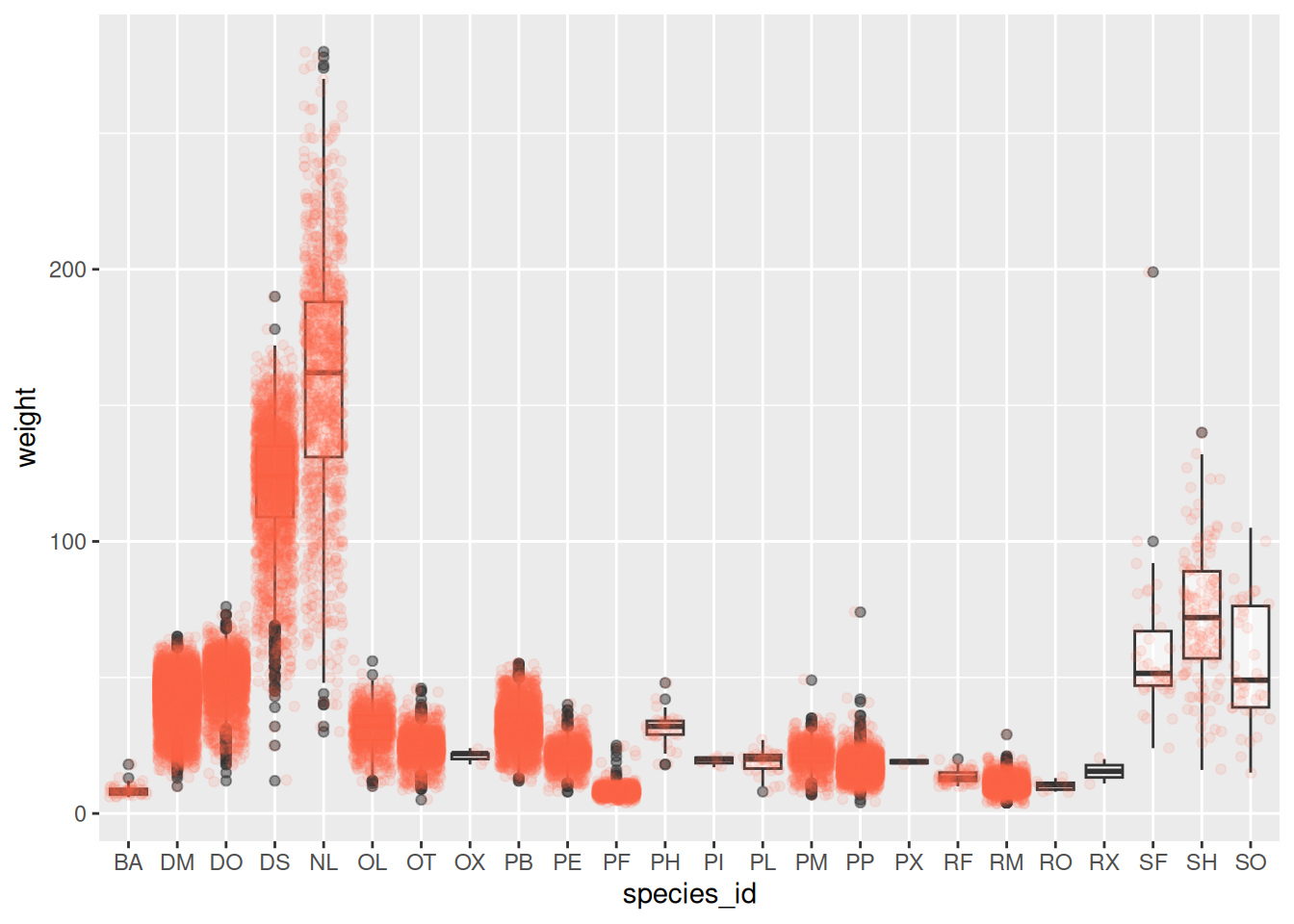
Boxplot

Time series data
# create appropriate dataset
yearly_count <- survey_complete %>%
  count(year, species_id)

surveys_plot <- ggplot(
  data = yearly_count,
  mapping = aes(x = year, y = n)
)

surveys_plot + geom_line()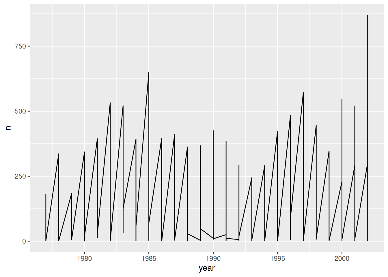
# make it more meaningful by breaking it by category
surveys_plot + geom_line(aes(group = species_id))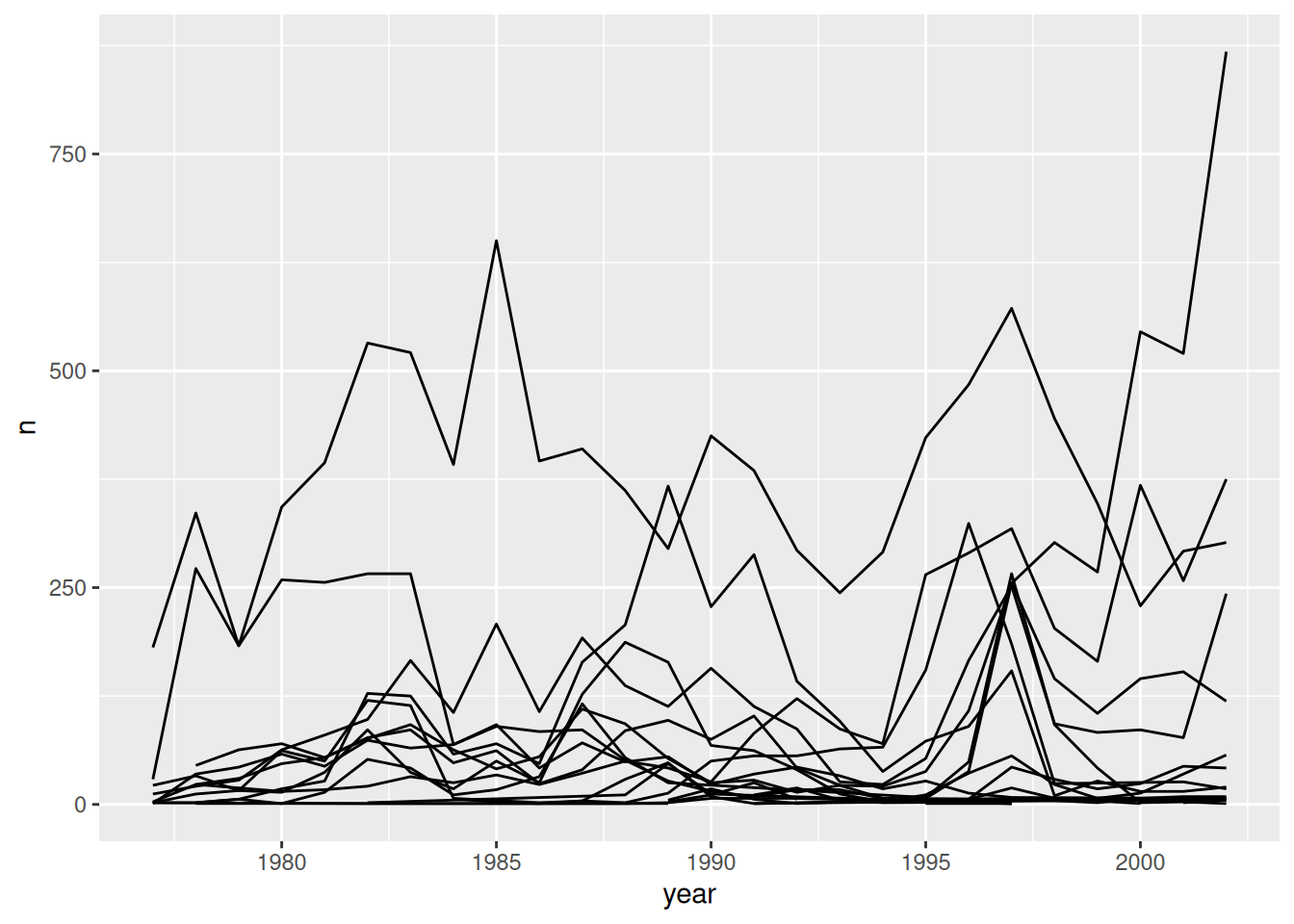
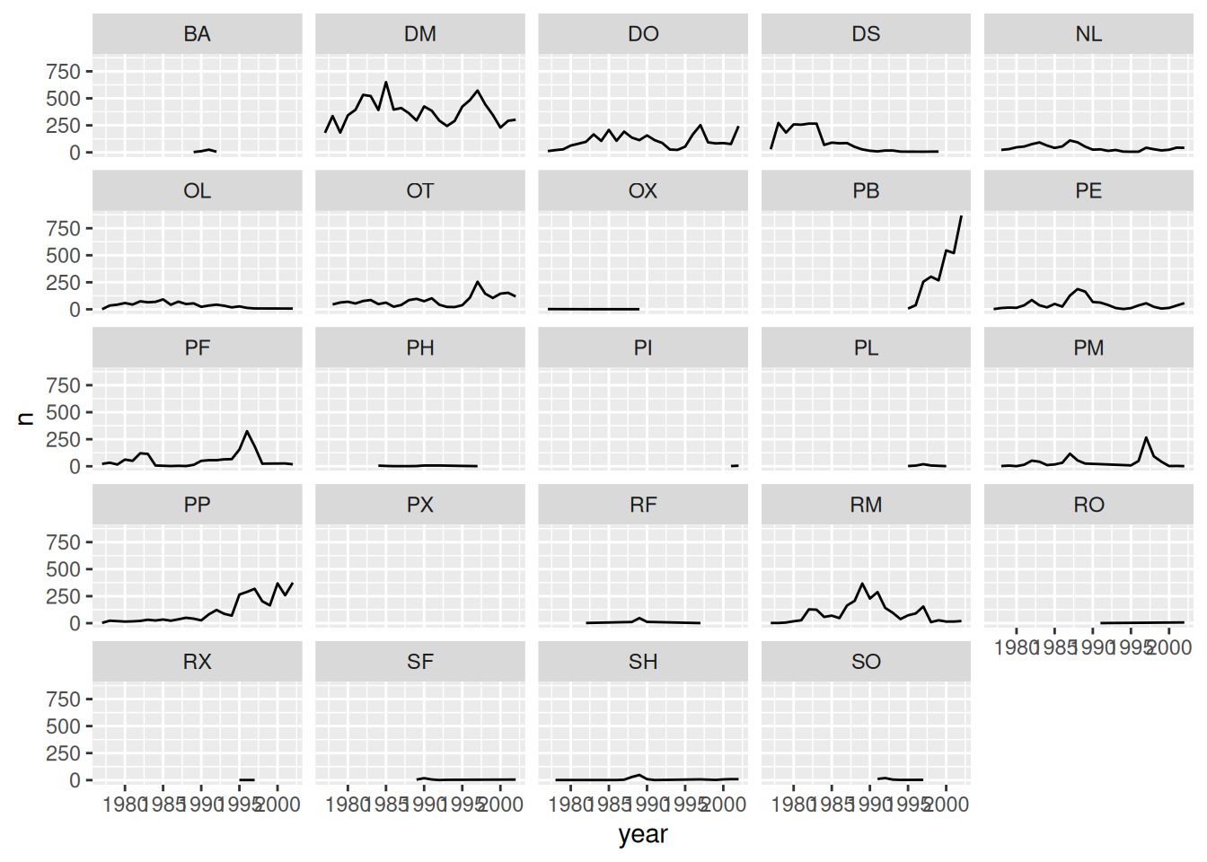
# split the line in each plot by sex
yearly_sex_counts <- survey_complete %>%
  count(year, species_id, sex)

surveys_plot <- ggplot(
  data = yearly_sex_counts,
  mapping = aes(x = year, y = n)
)

surveys_plot + geom_line(aes(color = sex)) +
  facet_wrap(~species_id)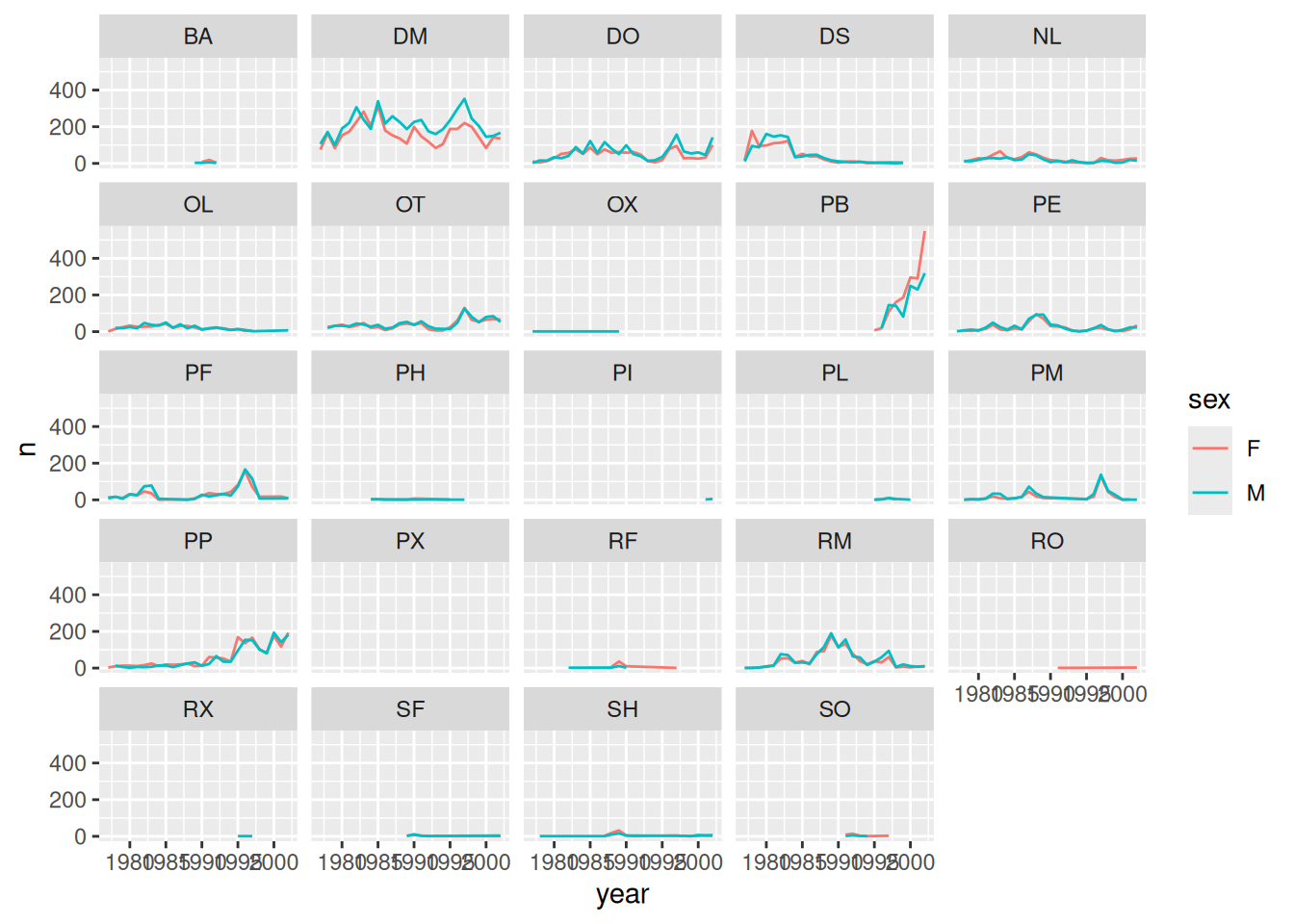
# remove background
surveys_plot + geom_line(aes(color = sex)) +
  facet_wrap(~species_id) +
  theme_bw() +
  theme(panel.grid = element_blank())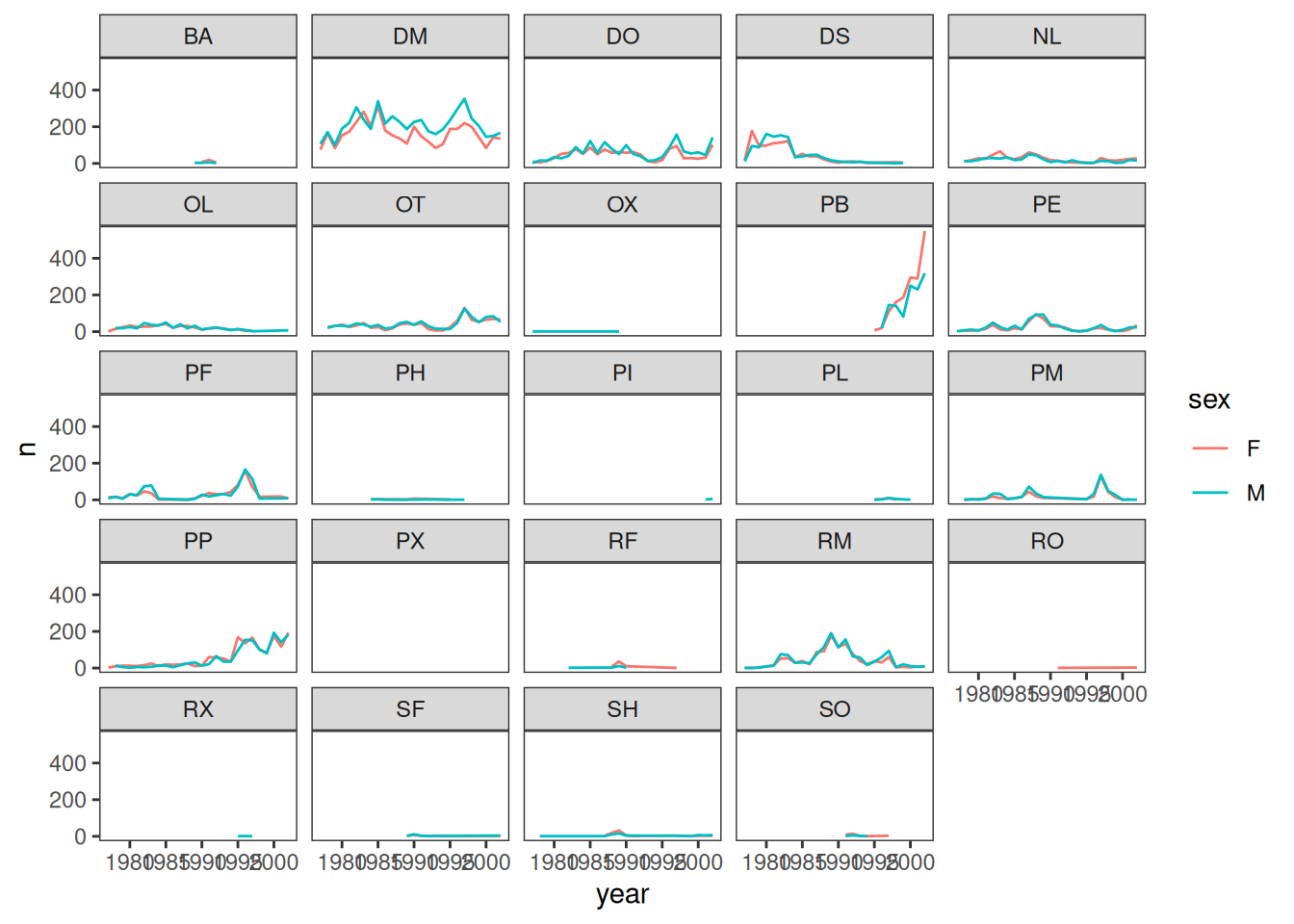
References
- OU Software Carpentry Workshop (check other workshops here)
- Intro to ggplot by Allison Horst
- R for Data Science book by Garrett Grolemund and Hadley Wickham
- Best Practices for Scientific Computing paper