Topic Modeling in R
Clear Workspace, DON’T EDIT
Always start by clearing the workspace. This ensure objects created in other files are not used used here.
List Used Packages, EDIT
List all the packages that will be used in chunk below.
Load Packages, DON’T EDIT
Install Missing
Any missing package will be installed automatically. This ensure smoother execution when run by others.
Be aware the people may not like installing packages into their machine automatically. This might break some of their previous code.
Load
Load all packages
Introduction
An attempt to understand Sherlock Holmes short stories found in Adventures of Sherlock Holmes book by Arthur Conan Doyle. After inspecting the table of content, the book seems to have 12 stories, one story per chapter. The analysis is inspired by Julia Silge’s YouTube video Topic modeling with R and tidy data principles
Download Book
# Download the book, each line of the book is read into a seperate row
sherlock_raw <- gutenberg_download(48320)
Determining mirror for Project Gutenberg from https://www.gutenberg.org/robot/harvestUsing mirror http://aleph.gutenberg.org[1] 12350 2# A tibble: 6 × 2
gutenberg_id text
<int> <chr>
1 48320 "ADVENTURES OF SHERLOCK HOLMES"
2 48320 ""
3 48320 ""
4 48320 ""
5 48320 ""
6 48320 "[Illustration:" # A tibble: 6 × 2
gutenberg_id text
<int> <chr>
1 48320 " boisterious fashion, and on the whole _changed to_"
2 48320 " boisterous fashion, and on the whole"
3 48320 ""
4 48320 " Page 297"
5 48320 " wrapt in the peaceful beauty _changed to_"
6 48320 " rapt in the peaceful beauty" Wrangle: Label Stories
sherlock <- sherlock_raw %>%

  # determine start of each story/chapter
  mutate(story = ifelse(str_detect(text, "^(A SCANDAL IN BOHEMIA|THE RED-HEADED LEAGUE|A CASE OF IDENTITY|THE BOSCOMBE VALLEY MYSTERY|THE FIVE ORANGE PIPS|THE MAN WITH THE TWISTED LIP|THE ADVENTURE OF THE BLUE CARBUNCLE|THE ADVENTURE OF THE SPECKLED BAND|THE ADVENTURE OF THE ENGINEER’S THUMB|THE ADVENTURE OF THE NOBLE BACHELOR|THE ADVENTURE OF THE BERYL CORONET|THE ADVENTURE OF THE COPPER BEECHES)$"), text, NA)) %>%

  # determine lines belonging to each story/chapter by
  # filling down the N/A rows of story column
  fill(story) %>%

  # remove the part that does not belong to any story/chapter,
  # i.e, the introduction
  filter(!is.na(story)) %>%

  # convert story column to factor
  mutate(story = factor(story))
Wrangle: Put in Tidy Format
The row of text column contains multiple words/tokens. We want to put each word/token of each text row into a separate row. This makes the dataframe follows the tidy format and hence makes it easy to process.
tidy_sherlock <- sherlock %>%

  # number the rows
  mutate(line = row_number()) %>%

  # break the text column into multiple row where each row contain one token
  unnest_tokens(word, text) %>%

  # remove the stopwords--the rows where the word column is a stopword
  anti_join(stop_words) %>%

  # remove holmes rows which might affect our topic models
  filter(word != "holmes")
Joining with `by = join_by(word)`Explore tf-idf
- To see which words are important in each story/chapter, i.e.,the words that appears many times in that story but few or none in the other stories.
- tf-idf (term frequency-inverse document frequency) is a great exploratory tool before starting with topic modeling
tidy_sherlock %>%

  # count number of occurrence of words in stories
  count(story, word, sort = TRUE) %>%

  # compute and add tf, idf, and tf_idf values for words
  bind_tf_idf(word, story, n) %>%

  # group by story
  group_by(story) %>%

  # take top 10 words of each story with highest tf_idf (last column)
  top_n(10) %>%

  # unpack
  ungroup() %>%

  # turn words into factors and order them based on their tf_idf values
  # NOTE: This will not affect order the dataframe rows which is can be
  #   done via the arrange function
  # NOTE: Recording the word column this way is for ggplot to visualize them
  #   as desired from top tf_idf to lowest
  mutate(word = reorder(word, tf_idf)) %>%

  # plot
  ggplot(aes(word, tf_idf, fill = story)) +
  geom_col(show.legend = FALSE) +
  facet_wrap(~story, scales = "free", ncol = 3) +
  theme(strip.text.x = element_text(size = 5)) +
  coord_flip()
Selecting by tf_idf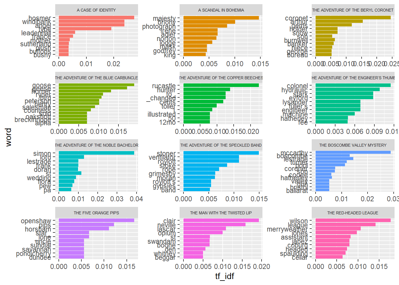
Implement Topic Modeling
Training the model for the topics
# Convert from tidy form to quanteda form (document x term matrix)
sherlock_stm <- tidy_sherlock %>%
  count(story, word, sort = TRUE) %>%
  cast_dfm(story, word, n)

# Train the model
topic_model <- stm(sherlock_stm, K=6, init.type = "Spectral")
Beginning Spectral Initialization
Calculating the gram matrix...
Finding anchor words...
......
Recovering initialization...
.............................................................................
Initialization complete.
............
Completed E-Step (0 seconds).
Completed M-Step.
Completing Iteration 1 (approx. per word bound = -7.785)
............
Completed E-Step (0 seconds).
Completed M-Step.
Completing Iteration 2 (approx. per word bound = -7.593, relative change = 2.458e-02)
............
Completed E-Step (0 seconds).
Completed M-Step.
Completing Iteration 3 (approx. per word bound = -7.481, relative change = 1.473e-02)
............
Completed E-Step (0 seconds).
Completed M-Step.
Completing Iteration 4 (approx. per word bound = -7.455, relative change = 3.469e-03)
............
Completed E-Step (0 seconds).
Completed M-Step.
Completing Iteration 5 (approx. per word bound = -7.450, relative change = 7.612e-04)
Topic 1: st, simon, lord, day, lady
Topic 2: door, miss, house, rucastle, matter
Topic 3: hat, goose, stone, bird, geese
Topic 4: father, time, mccarthy, son, hand
Topic 5: house, time, night, door, heard
Topic 6: red, time, wilson, business, headed
............
Completed E-Step (0 seconds).
Completed M-Step.
Completing Iteration 6 (approx. per word bound = -7.449, relative change = 1.233e-04)
............
Completed E-Step (0 seconds).
Completed M-Step.
Completing Iteration 7 (approx. per word bound = -7.449, relative change = 1.168e-05)
............
Completed E-Step (0 seconds).
Completed M-Step.
Model Converged A topic model with 6 topics, 12 documents and a 7709 word dictionary.Topic 1 Top Words:
Highest Prob: st, simon, lord, day, lady, found, matter
FREX: simon, clair, neville, lascar, opium, doran, flora
Lift: aloysius, ceremony, doran, millar, 2_s, aberdeen, absurdly
Score: simon, st, clair, neville, _danseuse_, lestrade, doran
Topic 2 Top Words:
Highest Prob: door, miss, house, rucastle, matter, street, lady
FREX: rucastle, hosmer, hunter, angel, windibank, _changed, 1
Lift: advertised, angel, annoyance, brothers, employed, factor, fowler
Score: rucastle, hosmer, angel, windibank, hunter, type, 1
Topic 3 Top Words:
Highest Prob: hat, goose, stone, bird, geese, baker, sir
FREX: geese, horner, ryder, henry, peterson, salesman, countess
Lift: battered, bet, bred, brixton, cosmopolitan, covent, cream
Score: goose, geese, horner, _alias_, ryder, henry, peterson
Topic 4 Top Words:
Highest Prob: father, time, mccarthy, son, hand, lestrade, left
FREX: mccarthy, pool, boscombe, openshaw, pips, horsham, turner
Lift: bone, dundee, horsham, pondicherry, presumption, savannah, sundial
Score: mccarthy, pool, lestrade, boscombe, openshaw, _détour_, turner
Topic 5 Top Words:
Highest Prob: house, time, night, door, heard, hand, round
FREX: coronet, stoner, arthur, roylott, ventilator, gems, stoke
Lift: _absolute_, _all_, _en, 1100, 16a, 3d, 4000
Score: coronet, arthur, stoner, gems, 4000, roylott, ventilator
Topic 6 Top Words:
Highest Prob: red, time, wilson, business, headed, day, league
FREX: wilson, league, merryweather, jones, coburg, jabez, headed
Lift: daring, saturday, vincent, _employé_, _october, _partie, 17
Score: wilson, league, merryweather, _employé_, jones, headed, coburg Contribution of Words in Topics
Looking at which words contribute the most in each topic.
# Extracting betas and putting them in a tidy format
tm_beta <- tidy(topic_model)

# Visualizing the top words contributing to each topic
tm_beta %>%
  group_by(topic) %>%
  # top 10 word in each topic with higest beta (last column)
  top_n(10) %>%
  ungroup() %>%
  # turn words into factors and order them based on their tf_idf values
  # NOTE: This will not affect order the dataframe rows which is can be
  #   done via the arrange function
  # NOTE: Recording the word column this way is for ggplot to visualize them
  #   as desired from top tf_idf to lowest
  mutate(term = reorder(term, beta)) %>%
  ggplot(aes(term, beta, fill = topic)) +
  geom_col(show.legend = FALSE) +
  facet_wrap(~topic, scales = "free", ncol = 3) +
  coord_flip()
Selecting by beta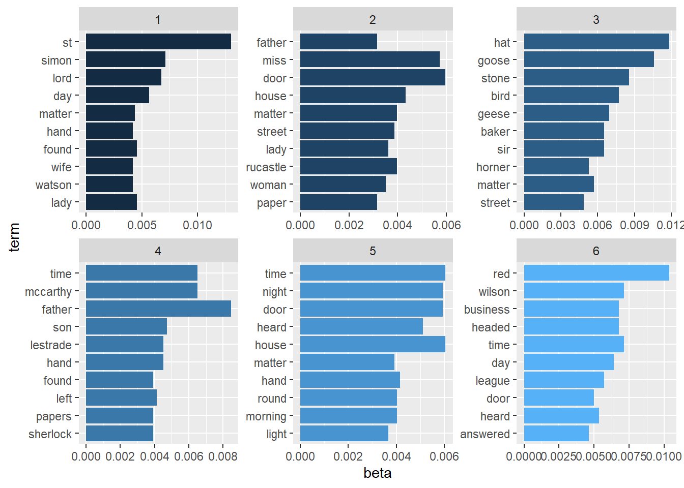
Distribution of Topics in Stories
Looking at how the stories are associated with each topic and how strong each association is.
# Extracting gammas and putting them in a tidy format
tm_gamma <- tidy(topic_model, matrix = "gamma",
                 # use the names of the stories instead of the default numbers
                 document_names = rownames(sherlock_stm))


# Visualizing the number of stories belonging to each topics and the confidence
#   of the belonging
tm_gamma %>%
  ggplot(aes(gamma, fill = as.factor(topic))) +
  geom_histogram(show.legend = FALSE) +
  facet_wrap(~topic, ncol = 3)
`stat_bin()` using `bins = 30`. Pick better value with `binwidth`.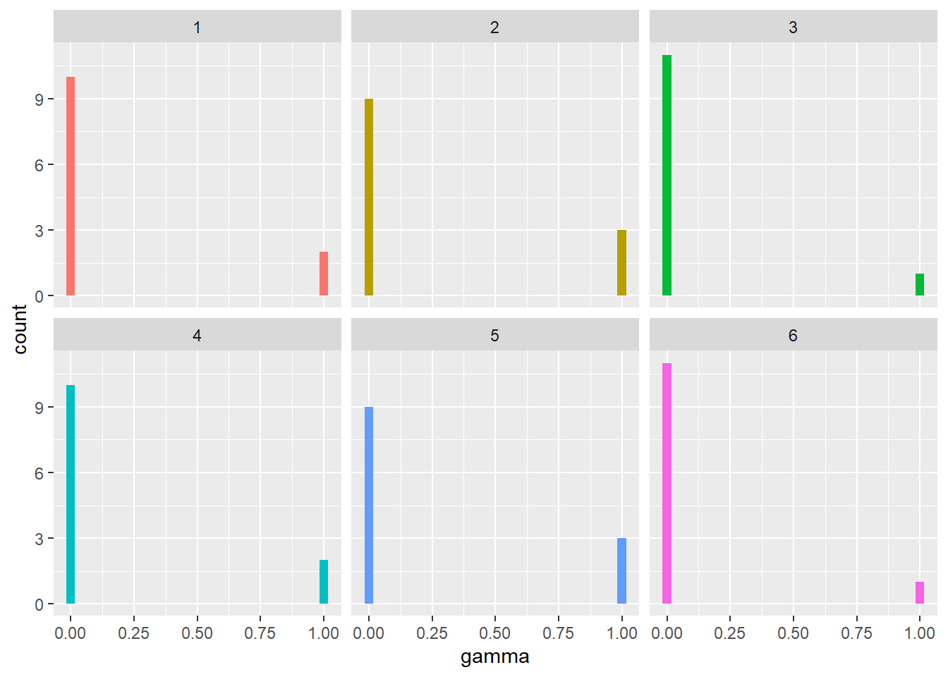
# Visualizing how much each topic appear in each story
tm_gamma %>%
  ggplot(aes(topic, gamma, fill = document)) +
  geom_col(show.legend = FALSE) +
  facet_wrap(~document, scales = "free", ncol = 3) +
  theme(strip.text.x = element_text(size = 5))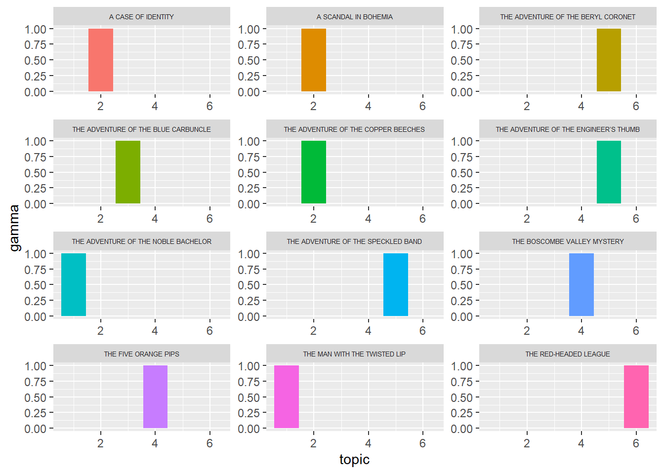
The model did an excellent job strongly associating the stories into one or more topics. This perfect association is rare in the world of topic modeling. The reason behind this perfect association here could be due to the small number of documents that we have.
References
- Adventures of Sherlock Holmes book by Arthur Conan Doyle on Project Gutenberg
- Regular Expressions 101