2 RStudio Workshop
Learning Goals
- Getting more familiar with RStudio
- Learn about a reproducible workflow in RStudio
- Work on Homework 1 with your group. The goals of the homework are:
- Explore tidy data
- Get familiar with RStudio
- Use Quarto to communicate reproducible document
Additional Resources
For more information about the topics covered in this chapter, refer to the resources below:
2.1 Warm-up
Background
What’s the point of this course?
Build knowledge from data within a particular domain of inquiry, and particular contexts.
Why will we use R/RStudio as a tool in this course?
- It’s open access, ie, free!
- It’s open source, ie, anyone can contribute to its development
- It’s used broadly–here are some examples where R is used:
- Logan Pratico: making “eviction data accessible to the legal aid community”
- Ahmadou Dicko: humanitarians creating “life saving data products”
- Shelmith Kariuki: Kenyan government census
- Laura DeCicco: U.S. Geological Survey (USGS) discovery and retrieval of hydrologic data
- Nick Snellgrove & Uli Muellner: studying aquatic invasive species in MN
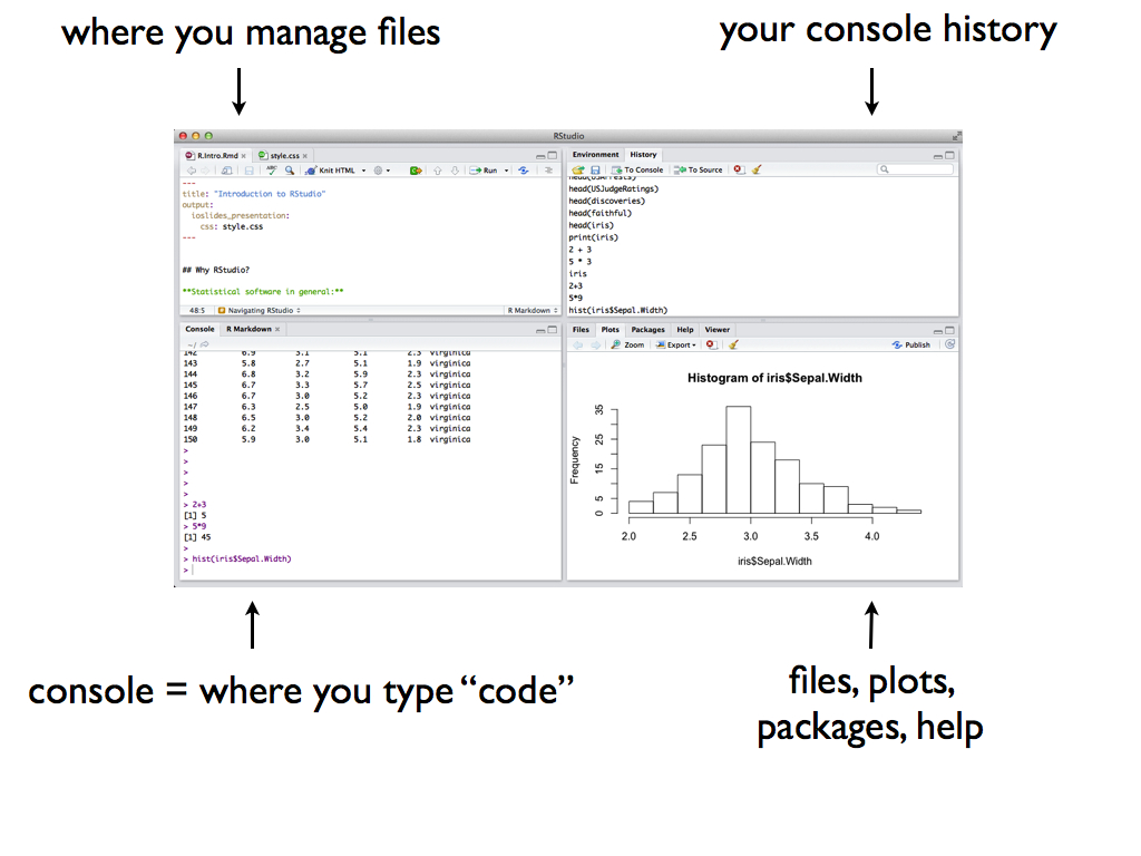
RStudio Layout
Below is a screenshot of the default layout for RStudio.
Console
Last class, we spent most of our time in the console. However,
| Console is good for… | Console is bad for most everything else, including… |
|---|---|
| quick calculations | documenting our work |
| trying out code | editing our work |
| pulling up help files | communicating our work |
| being able to reproduce our work |
Quarto
Reproducibility with Quarto
It’s important to document and communicate every step in the data analysis process, e.g. data collection, cleaning, and analysis, so that others and ourselves can reproduce and hence verify and build upon our work.
RStudio includes tools for creating reproducible and lovely documents, webpages, books (like this online manual!), etc that allow us to interleave text, code, output, images, tables, etc. Quarto is integrated into RStudio and if you’ve used R Markdown, it looks very similar.
Quarto
Quarto is an technology that incorporates code from many programming languages such as R along with styled text (headers, bold, italics, links, etc.) using markdown.
Quarto Example
Download then move this Quarto document into the activities folder of your portfolio project and do not forgot to include it in _quarto.yml file. Open the Quarto document in RStudio and follow the prompts therein. Note that this document explores the basics. We’ll pick up more details as we go, often by making and learning from mistakes. The Quarto cheatsheets linked at the top of this chapter presents more features of Quarto.
Important Tips
Quarto Files (.qmd) vs Console
The console does not communicate with Quarto. Things you define or type in the console are NOT defined, stored, or run in the .qmd.
-
Quarto can communicate with the console, but only if you tell it to.
- IT WILL: if you run a chunk inside your .qmd (by clicking the green arrow), it is also run and stored in the console.
- IT WON’T: if you render your .qmd to html but do not also run the chunks inside the .qmd, the results will be displayed in the html but not run or stored in the console.
Styling Guides
All of this emphasis on communication is not specific to this class, it is a general expectation. Further, the code structure we’ll use this semester reflects common practice, but not the only practice. Various companies / entities have their own R “style guides”. Below are two examples of such styling guides.
-
tidyverse style guide
- R developers like using the snake_case when naming variables
-
Google’s R Style Guide
- Google on the other hand recommends using the camelCase when naming variables
2.2 Homework 1
Instructions, Reminder
- The following exercises will be due as homework 1.
- You should work on these exercises in groups, but write up your own work.
Getting Started
For most homeworks and in-class activities, you will be provided with a Quarto (.qmd) template. However, it’s also important to practice starting your own Quarto .qmd from scratch. You’ll do that here.
Instructions
Before starting the exercises, take the following steps:
Follow the instructions on Appendix: Submitting Homeworks to create your homework repository
In the homeworks folder of your cloned repository, create a new Quarto (.qmd) file: File window in the lower-right corner –> Add New File (second icon from the left) –> Quarto Doc… –> name it
homework_01.qmdEdit the
_quarto.ymlfile to include the document-
In the newly created document, add the following YAML header at the top. The YAML option
number-sectionswill prevent numbering the headers of the documents. -
Below the yaml header, add section headers for each homework exercise as follows:
Render the book to html by clicking Render Book button in the Build located in the upper-right section.
Put your answers to each exercise under the appropriate
# Exercisesection. You do not need to write out the question/prompt itself.
Exercise 1: Warming Up
- Write 1 sentence about one of your favorite foods at Cafe Mac. Make sure to include an italicized word and a bold word.
- Show a .png image of the food from the web. In Google, you can add
filetype:pngto the beginning of your search term, click on the photo you want, and copy the image address.
Check → Commit → Push
Before continuing, click Render Book again and make sure it looks like what you want. If happy, jump to GitHub Desktop and commit the changes with the message Finish HW1 Ex1 and push to GitHub.
Exercise 2: Import Tidy Data
A quick survey was filled before class. So, let’s work with this data. The first step to working with data in RStudio is getting it in there which depends on:
- file format, eg,
.xls(Excel spreadsheet),.csv, or.txt - storage locations, eg, online, on your desktop, or built into RStudio itself.
Our data is stored as a .csv file online. Within a new R chunk, import and store this data as survey. Take note of the function name and the argument it takes.
Note that nothing new appears in your document after you import the data. This is because we stored, but didn’t print, the data. Actually, we don’t want to print the data in our .qmd file–it would be too messy.
There are 2 quick ways to check out the entire data table to get a sense of its structure and contents:
- Type
View(survey)in the console. - In the Environment tab (upper right pane), click on
survey.
Check → Commit → Push
Before continuing, click Render Book again and make sure it looks like what you want. If happy, jump to GitHub Desktop and commit the changes with the message Finish HW1 Ex2 and push to GitHub.
Exercise 3: Tidy Data Properties
Answers the following prompts in a bulleted list in the order they’re presented.
- What are the units of observation, ie, what does each row represent?
- Name one quantitative variable, ie, column, in the dataset.
- Name one categorical variable, ie, column, in the dataset.
Creating Bulleted List
To create a bulleted list, use - in front of each item and make sure to leave an empty line before the list.
Check → Commit → Push
Before continuing, click Render Book again and make sure it looks like what you want. If happy, jump to GitHub Desktop and commit the changes with the message Finish HW1 Ex3 and push to GitHub.
Exercise 4: Know the Data
Before we can learn anything from our data, we must understand its structure. For each function below, try out one at a time then write a short comment/note about what the function does in the indicated places. To make for easier recall later, try to connect your comment on what the function does to how it’s named.
# Replace this with a comment on what dim() does
dim(survey)

# Replace this with a comment on what nrow() does
nrow(survey)

# Replace this with a comment on what head() does
head(survey)

# Replace this with a comment on what head(___, 3) does
head(survey, 3)

# Replace this with a comment on what tail() does
tail(survey)

# Replace this with a comment on what names() does
names(survey)
Check → Commit → Push
Before continuing, click Render Book again and make sure it looks like what you want. If happy, jump to GitHub Desktop and commit the changes with the message Finish HW1 Ex4 and push to GitHub.
Exercise 5: Data Structure
It’s important that we understand the different types or structures of the objects we store. Having such information will inform what types of analyses are appropriate and the appropriate R code for these analyses. The class() function is important here. The example below shows how it can be used and what output it produces.
There are various object classes, including:
-
numornumeric -
intorinteger -
chrorcharacter -
factor, and -
data.frame.
Complete the chunk below to explore the classes/structure of our survey data and the variables within the survey data:
Check → Commit → Push
Before continuing, click Render Book again and make sure it looks like what you want. If happy, jump to GitHub Desktop and commit the changes with the message Finish HW1 Ex5 and push to GitHub.
Exercise 6: Your turn
Let’s practice these same ideas using data on World Cup football/soccer found on:
https://raw.githubusercontent.com/rfordatascience/tidytuesday/master/data/2022/2022-11-29/worldcups.csv
Data is only useful if we know what it’s measuring! You can find a codebook, i.e. document that describes the data, here. Address each prompt below using R functions. Include both the # prompt and your code in the chunk.
# Import and name the dataset (you pick a name!)


# Print the first 6 rows of the dataset


# How many years of data do we have? And how many measurements do we have on each year?


# Get a list of all variable names in the dataset


# Display the class and other information for each variable in the dataset
Check → Commit → Push
Before continuing, click Render Book again and make sure it looks like what you want. If happy, jump to GitHub Desktop and commit the changes with the message Finish HW1 Ex6 and push to GitHub.
Exercise 7: Brainstorm
We’ve just scratched the surface. In a bulleted list (-), write out 3 questions about the World Cup that we might answer using these data. Be creative. The questions don’t have to be questions we’ve learned how to answer yet.
Check → Commit → Push
Before continuing, click Render Book again and make sure it looks like what you want. If happy, jump to GitHub Desktop and commit the changes with the message Finish HW1 Ex7 and push to GitHub.
Check GitHub
Go to your repository on GitHub (GitHub Desktop → Repository menu item → View on GitHub) and make sure that all your commits are there.
Congratulation 🎉. You’re done with Homework 1.
Optional: More Challenges
If you like to do more, here are some things to think about–this will be different from student to student based on current R experience, post-graduate goals, interests, etc.
If you are thinking about communication including aesthetics:
- Check out other features of Quarto, shown in the Quarto Start up Guide linked at the top of this chapter
- Check out the different themes or ways you might style a Quarto document.
- Check out this gallery of Quarto websites (and other documents) and learn how to build Quarto websites right from RStudio.
If you are thinking about data, there are many places where you can get some. Actually, the World Cup data came from a weekly social data project called TidyTuesday. TidyTuesday is a community of R users from around the globe who share and dig into one different dataset per week then share their results in various channels such as YouTube and social media. Check out the repository of the TidyTuesday datasets at https://github.com/rfordatascience/tidytuesday. In the DataSets section, click on the year and then scroll down to a table of datasets posted that year. Pick a dataset of interest, import this into R, and play around! Be creative.
Lisa Lendway is a Mac alum, former Mac prof who helped shape this course, and R/RStudio whiz.↩︎
Comments
Leaving short notes (known as comments) about what our code is doing is an important aspect of communication. It reminds our future selves, and communicates to others, what our thought and code process was. Hence comments are important to reproducibility. In the R chunks, comments are proceeded by a pound sign:
# This is an example comment.