10  Reshaping Data

Learning Goals

• Understand what it means to “reshape” data.
• Understand the difference between wide and long data formats.
• Be able to distinguish the units of observation for a given data set.
• Explore how to reshape data using pivot_wider() and pivot_longer() in the tidyr package

Additional Resources

For more information about the topics covered in this chapter, refer to the resources below:

• Demonstrating pivoting (YouTube) by Lisa Lendway
• Pivoting vignette (html) by tidyr
• Pivoting (html) by Wickham and Grolemund
• Reshaping data by Baumer, Kaplan, and Horton

Instructions

General

• Be kind to yourself.
• Collaborate with and be kind to others. You are expected to work together as a group.
• Ask questions. Remember that we won’t discuss these exercises as a class.

Activity Specific

Help each other with the following:

• Create a new Quarto document in the activities folder of your portfolio project and do not forgot to include it in _quarto.yml file. Then click the </> Code link at the top right corner of this page and copy the code into the created Quarto document. This is where you’ll take notes. Remember that the portfolio is yours, so take notes in whatever way is best for you.
• Don’t start the Exercises section before we get there as a class. First, engage in class discussion and eventually collaborate with your group on the exercises!

10.1 Warm-up

EXAMPLE 1: warm-up counts and proportions

Recall the penguins we worked with last class:

library(tidyverse)
penguins <- read_csv('https://raw.githubusercontent.com/rfordatascience/tidytuesday/master/data/2020/2020-07-28/penguins.csv')

Tally up the number of male/female penguins by species in 2 ways:

# Using count()


# Using group_by() and summarize()

Define a new column that includes the proportion or relative frequencies of male/female penguins in each species.

• We can’t do this by adjusting our count() code, but can adjust the group_by() and summarize() code since it’s still tracking the group categories in the background.
• Does the order of species and sex in group_by() matter?

EXAMPLE 2: New data

What will the following code do? Think about it before running.

penguin_avg <- penguins |> 
  group_by(species, sex) |> 
  summarize(avg_body_mass = mean(body_mass_g, na.rm = TRUE)) |> 
  na.omit()

EXAMPLE 3: units of observation

To get the information on average body masses, we reshaped our original data.

1. Did the reshaping process change the units of observation?

# Units of observation = ???
head(penguins)

# A tibble: 6 × 8
  species island    bill_length_mm bill_depth_mm flipper_length_mm body_mass_g
  <chr>   <chr>              <dbl>         <dbl>             <dbl>       <dbl>
1 Adelie  Torgersen           39.1          18.7               181        3750
2 Adelie  Torgersen           39.5          17.4               186        3800
3 Adelie  Torgersen           40.3          18                 195        3250
4 Adelie  Torgersen           NA            NA                  NA          NA
5 Adelie  Torgersen           36.7          19.3               193        3450
6 Adelie  Torgersen           39.3          20.6               190        3650
# ℹ 2 more variables: sex <chr>, year <dbl>

# Units of observation = ???
head(penguin_avg)

# A tibble: 6 × 3
# Groups:   species [3]
  species   sex    avg_body_mass
  <chr>     <chr>          <dbl>
1 Adelie    female         3369.
2 Adelie    male           4043.
3 Chinstrap female         3527.
4 Chinstrap male           3939.
5 Gentoo    female         4680.
6 Gentoo    male           5485.

2. Did the reshaping process result in any information loss from the original data?

Reshaping data

There are two general types of reshaped data:

• aggregate data
  For example, using group_by() with summarize() gains aggregate information about our observations but loses data on individual observations.

• raw data, reshaped
  We often want to retain all information on individual observations, but need to reshape it in order to perform the task at hand.

EXAMPLE 4: reshape it with your mind

Let’s calculate the difference in average body mass, male vs female, for each species. Since penguin_avg is small, we could do these calculations by hand. But this doesn’t scale up to bigger datasets.

• Sketch out (on paper, in your head, anything) how this data would need to be reshaped, without losing any information, in order to calculate the differences in average body mass using our wrangling verbs. Make it as specific as possible, with column labels, entries, correct numbers, etc.

• Identify the units of observation.

penguin_avg

# A tibble: 6 × 3
# Groups:   species [3]
  species   sex    avg_body_mass
  <chr>     <chr>          <dbl>
1 Adelie    female         3369.
2 Adelie    male           4043.
3 Chinstrap female         3527.
4 Chinstrap male           3939.
5 Gentoo    female         4680.
6 Gentoo    male           5485.

Wider vs Longer formats

Making our data longer or wider reshapes the data, changing the units of observation while retaining all raw information:

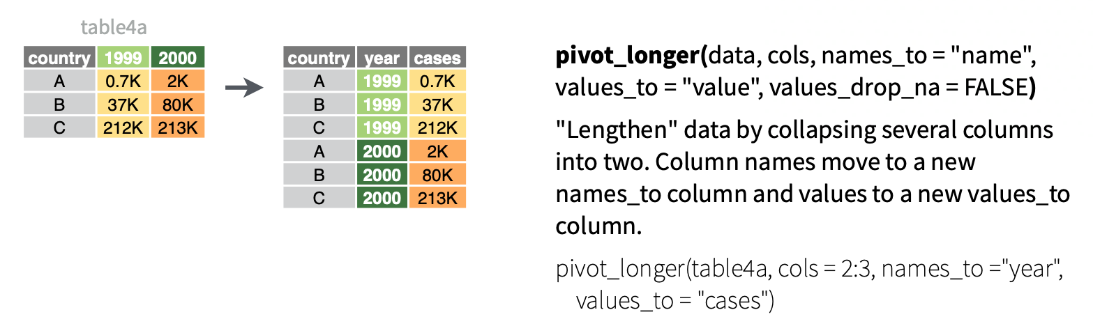
1. Make the data longer, i.e. combine values from multiple variables into 1 variable. EXAMPLE: 1999 and 2000 represent two years. We want to combine their results into 1 variable without losing any information.

2. Make the data wider, i.e. spread out the values across new variables. EXAMPLE: cases and pop represent two categories within type. To compare or combine their count outcomes side-by-side, we can separate them into their own variables.

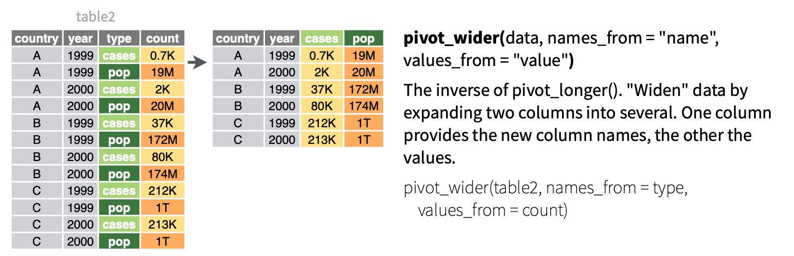
EXAMPLE 5: pivot wider

Because it’s a small enough dataset to examine all at once, let’s start with our penguin_avg data:

penguin_avg

# A tibble: 6 × 3
# Groups:   species [3]
  species   sex    avg_body_mass
  <chr>     <chr>          <dbl>
1 Adelie    female         3369.
2 Adelie    male           4043.
3 Chinstrap female         3527.
4 Chinstrap male           3939.
5 Gentoo    female         4680.
6 Gentoo    male           5485.

With the goal of being able to calculate the difference in average body mass, male vs female, for each species, let’s make the dataset wider. That is, let’s get one row per species with separate columns for the average body mass by sex. Put this code into a chunk and run it:

penguin_avg |> pivot_wider(names_from = sex, values_from = avg_body_mass)

Pivot Wider

• names_from = the variable whose values we want to separate into their own columns, i.e. where we want to get the new column names from
• values_from = which variable to take the new column values from

FOLLOW-UP:

• What are the units of observation?

• Did we lose any information when we widened the data?

• Use the wide data to calculate the difference in average body mass, male vs female, for each species.

EXAMPLE 6: Pivot longer

Let’s store our wide data:

penguin_avg_wide <- penguin_avg |> 
  pivot_wider(names_from = sex, values_from = avg_body_mass)

penguin_avg_wide

# A tibble: 3 × 3
# Groups:   species [3]
  species   female  male
  <chr>      <dbl> <dbl>
1 Adelie     3369. 4043.
2 Chinstrap  3527. 3939.
3 Gentoo     4680. 5485.

Suppose we wanted to change this data back to a longer format. In general, this happens when some variables (here female and male) represent two categories or values of some broader variable (here sex), and we want to combine them into that 1 variable without losing any information. Let’s pivot_longer():

# We can either communicate which variables we WANT to collect into a single column (female, male)
penguin_avg_wide |> 
  pivot_longer(cols = c(female, male), names_to = "sex", values_to = "avg_body_mass")

# A tibble: 6 × 3
# Groups:   species [3]
  species   sex    avg_body_mass
  <chr>     <chr>          <dbl>
1 Adelie    female         3369.
2 Adelie    male           4043.
3 Chinstrap female         3527.
4 Chinstrap male           3939.
5 Gentoo    female         4680.
6 Gentoo    male           5485.

# Or which variable(s) we do NOT want to collect into a single column (sex)
penguin_avg_wide |> 
  pivot_longer(cols = -species, names_to = "sex", values_to = "avg_body_mass")

# A tibble: 6 × 3
# Groups:   species [3]
  species   sex    avg_body_mass
  <chr>     <chr>          <dbl>
1 Adelie    female         3369.
2 Adelie    male           4043.
3 Chinstrap female         3527.
4 Chinstrap male           3939.
5 Gentoo    female         4680.
6 Gentoo    male           5485.

Pivot Longer

• cols = the columns (variables) to collect into a single, new variable. we can also specify what variables we don’t want to collect
• names_to = the name of the new variable which will include the names or labels of the collected variables
• values_to = the name of the new variable which will include the values of the collected variables

FOLLOW-UP:

• What are the units of observation?

• Did we lose any information when we lengthened the data?

• Why did we put the variables in quotes “” here but not when we used pivot_wider()?

EXAMPLE 7: Practice

Let’s make up some data on the orders of 2 different customers at 3 different restaurants:

food <- data.frame(
  customer = rep(c("A", "B"), each = 3),
  restaurant = rep(c("Shish", "FrenchMeadow", "DunnBros"), 2),
  order = c("falafel", "salad", "coffee", "baklava", "pastry", "tea")
)
food

  customer   restaurant   order
1        A        Shish falafel
2        A FrenchMeadow   salad
3        A     DunnBros  coffee
4        B        Shish baklava
5        B FrenchMeadow  pastry
6        B     DunnBros     tea

The units of observation in food are customer / restaurant combinations. Wrangle this data so that the units of observation are customers, spreading the restaurants into separate columns.

Consider 2 more customers:

more_food <- data.frame(
  customer = c("C", "D"),
  Shish = c("coffee", "maza"),
  FrenchMeadow = c("soup", "sandwich"),
  DunnBros = c("cookie", "coffee")
)
more_food

  customer  Shish FrenchMeadow DunnBros
1        C coffee         soup   cookie
2        D   maza     sandwich   coffee

Wrangle this data so that the 3 restaurant columns are combined into 1, hence the units of observation are customer / restaurant combinations.

10.2 Exercises

Exercise 1: What’s the problem?

Consider data on a sleep study in which subjects received only 3 hours of sleep per night. Each day, their reaction time to a stimulus (in ms) was recorded.¹

sleep_wide <- read.csv("https://mac-stat.github.io/data/sleep_wide.csv")

head(sleep_wide)

  Subject  day_0  day_1  day_2  day_3  day_4  day_5  day_6  day_7  day_8  day_9
1     308 249.56 258.70 250.80 321.44 356.85 414.69 382.20 290.15 430.59 466.35
2     309 222.73 205.27 202.98 204.71 207.72 215.96 213.63 217.73 224.30 237.31
3     310 199.05 194.33 234.32 232.84 229.31 220.46 235.42 255.75 261.01 247.52
4     330 321.54 300.40 283.86 285.13 285.80 297.59 280.24 318.26 305.35 354.05
5     331 287.61 285.00 301.82 320.12 316.28 293.32 290.08 334.82 293.75 371.58
6     332 234.86 242.81 272.96 309.77 317.46 310.00 454.16 346.83 330.30 253.86

Part a

What are the units of observation in sleep_wide?

Part b

Suppose I ask you to plot each subject’s reaction time (y-axis) vs the number of days of sleep restriction (x-axis). “Sketch” out in words what the first few rows of the data need to look like in order to do this. It might help to think about what you’d need to complete the plotting frame:

ggplot(___, aes(y = ___, x = ___, color = ___))

Part c

How can you obtain the dataset you sketched in part b?

• just using sleep_wide
• pivot_longer()
• pivot_wider()

Exercise 2: Pivot longer

To plot reaction time by day for each subject, we need to reshape the data into a long format where each row represents a subject/day combination. Specifically, we want a dataset with 3 columns and a first few rows that look something like this:

Subject	day	reaction_time
308	0	249.56
308	1	258.70
308	2	250.80

Part a

Use pivot_longer() to create the long-format dataset above. Show the first 3 lines (head(3)), which should be similar to those above. Follow-up: Thinking forward to plotting reaction time vs day for each subject, what would you like to fix / change about this dataset?

# For cols, try 2 appproaches: using - and starts_with
# ___ |> 
#   pivot_longer(cols = ___, names_to = "___", values_to = "___")

Part b

Run this chunk:

sleep_long <- sleep_wide |>
  pivot_longer(cols = -Subject,
               names_to = "day",
               names_prefix = "day_",
               values_to = "reaction_time")

head(sleep_long)

# A tibble: 6 × 3
  Subject day   reaction_time
    <int> <chr>         <dbl>
1     308 0              250.
2     308 1              259.
3     308 2              251.
4     308 3              321.
5     308 4              357.
6     308 5              415.

Follow-up:

• Besides putting each argument on a different line for readability and storing the results, what changed in the code?
• How did this impact how the values are recorded in the day column?

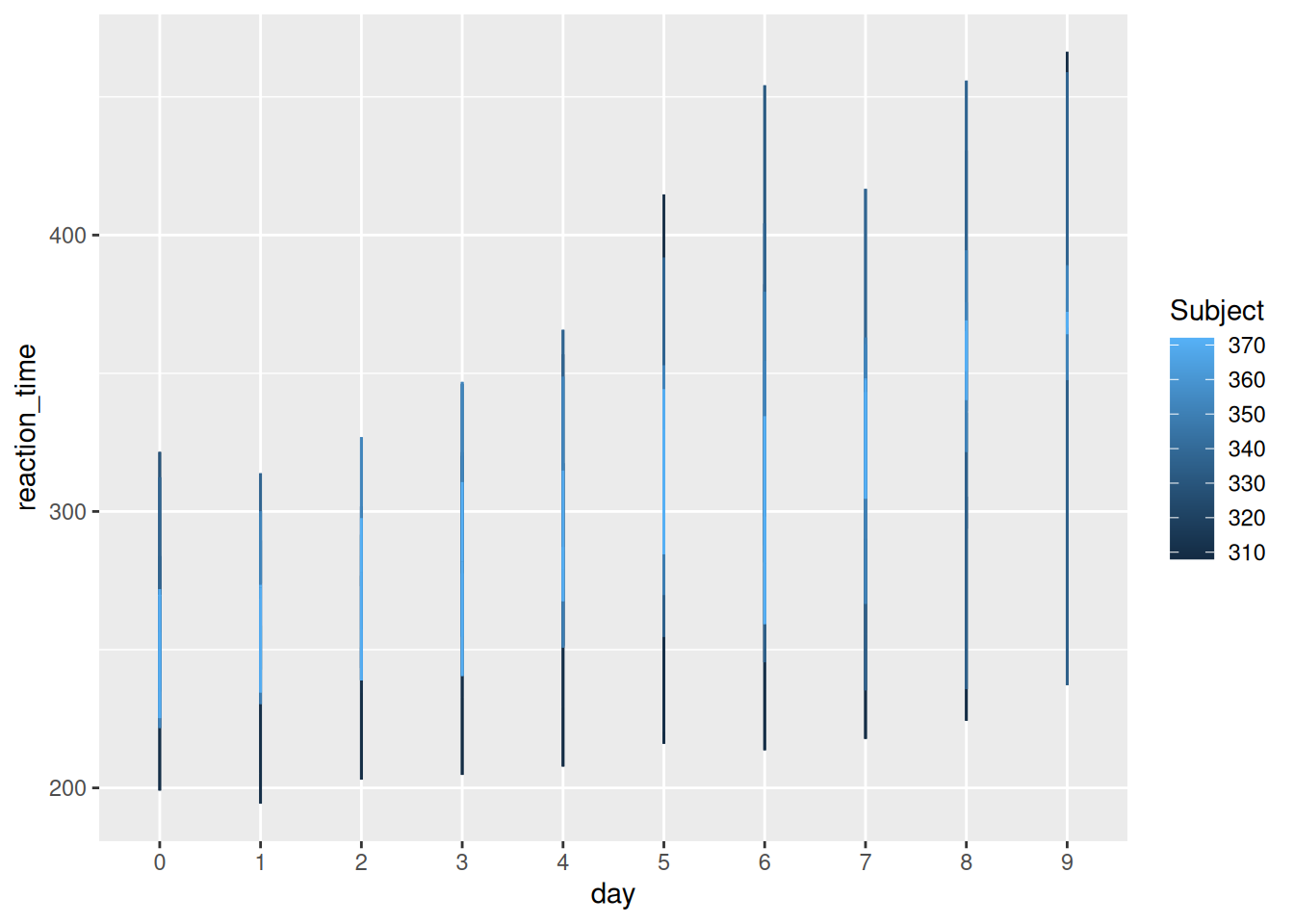
Part c

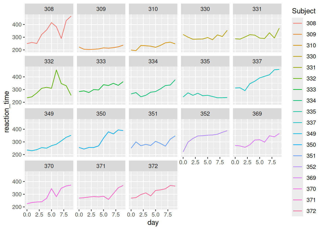
Using sleep_long, construct a line plot of reaction time vs day for each subject. This will look goofy no matter what you do. Why? HINT: look back at head(sleep_long). What class or type of variables are Subject and day? What do we want them to be?

Exercise 3: Changing variable classes & plotting

Let’s finalize sleep_long by mutating the Subject variable to be a factor (categorical) and the day variable to be numeric (quantitative). Take note of the mutate() code! You’ll use this type of code a lot.

sleep_long <- sleep_wide |>
  pivot_longer(cols = -Subject,
               names_to = "day",
               names_prefix = "day_",
               values_to = "reaction_time") |> 
  mutate(Subject = as.factor(Subject), day = as.numeric(day))

# Check it out
# Same data, different class
head(sleep_long)

# A tibble: 6 × 3
  Subject   day reaction_time
  <fct>   <dbl>         <dbl>
1 308         0          250.
2 308         1          259.
3 308         2          251.
4 308         3          321.
5 308         4          357.
6 308         5          415.

Part a

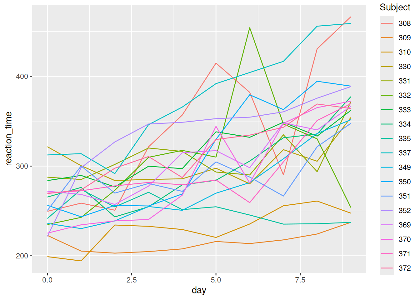
Now make some plots.

# Make a line plot of reaction time by day for each subject
# Put these all on the same frame

# Make a line plot of reaction time by day for each subject
# Put these all on separate frames (one per subject)

Part b

Summarize what you learned from the plots. For example:

• What’s the general relationship between reaction time and sleep?
• Is this the same for everybody? What differs?

Exercise 4: Pivot wider

Make the data wide again, with each day becoming its own column.

Part a

Adjust the code below. What don’t you like about the column labels?

# sleep_long |>
#   pivot_wider(names_from = ___, values_from = ___) |> 
#   head()

Part b

Using your intuition, adjust your code from part a to name the reaction time columns “day_0”, “day_1”, etc.

# sleep_long |>
#   pivot_wider(names_from = ___, values_from = ___, names_prefix = "___") |> 
#   head()

Exercise 5: Practice with Billboard charts

Load data on songs that hit the billboard charts around the year 2000. Included for each song is the artist name, track name, the date it hit the charts (date.enter), and wk-related variables that indicate rankings in each subsequent week on the charts:

# Load data
library(tidyr)
data("billboard")

# Check it out
head(billboard)

# A tibble: 6 × 79
  artist      track date.entered   wk1   wk2   wk3   wk4   wk5   wk6   wk7   wk8
  <chr>       <chr> <date>       <dbl> <dbl> <dbl> <dbl> <dbl> <dbl> <dbl> <dbl>
1 2 Pac       Baby… 2000-02-26      87    82    72    77    87    94    99    NA
2 2Ge+her     The … 2000-09-02      91    87    92    NA    NA    NA    NA    NA
3 3 Doors Do… Kryp… 2000-04-08      81    70    68    67    66    57    54    53
4 3 Doors Do… Loser 2000-10-21      76    76    72    69    67    65    55    59
5 504 Boyz    Wobb… 2000-04-15      57    34    25    17    17    31    36    49
6 98^0        Give… 2000-08-19      51    39    34    26    26    19     2     2
# ℹ 68 more variables: wk9 <dbl>, wk10 <dbl>, wk11 <dbl>, wk12 <dbl>,
#   wk13 <dbl>, wk14 <dbl>, wk15 <dbl>, wk16 <dbl>, wk17 <dbl>, wk18 <dbl>,
#   wk19 <dbl>, wk20 <dbl>, wk21 <dbl>, wk22 <dbl>, wk23 <dbl>, wk24 <dbl>,
#   wk25 <dbl>, wk26 <dbl>, wk27 <dbl>, wk28 <dbl>, wk29 <dbl>, wk30 <dbl>,
#   wk31 <dbl>, wk32 <dbl>, wk33 <dbl>, wk34 <dbl>, wk35 <dbl>, wk36 <dbl>,
#   wk37 <dbl>, wk38 <dbl>, wk39 <dbl>, wk40 <dbl>, wk41 <dbl>, wk42 <dbl>,
#   wk43 <dbl>, wk44 <dbl>, wk45 <dbl>, wk46 <dbl>, wk47 <dbl>, wk48 <dbl>, …

In using this data, you’ll need to determine if and when the data needs to be reshaped for the task at hand.

Part a

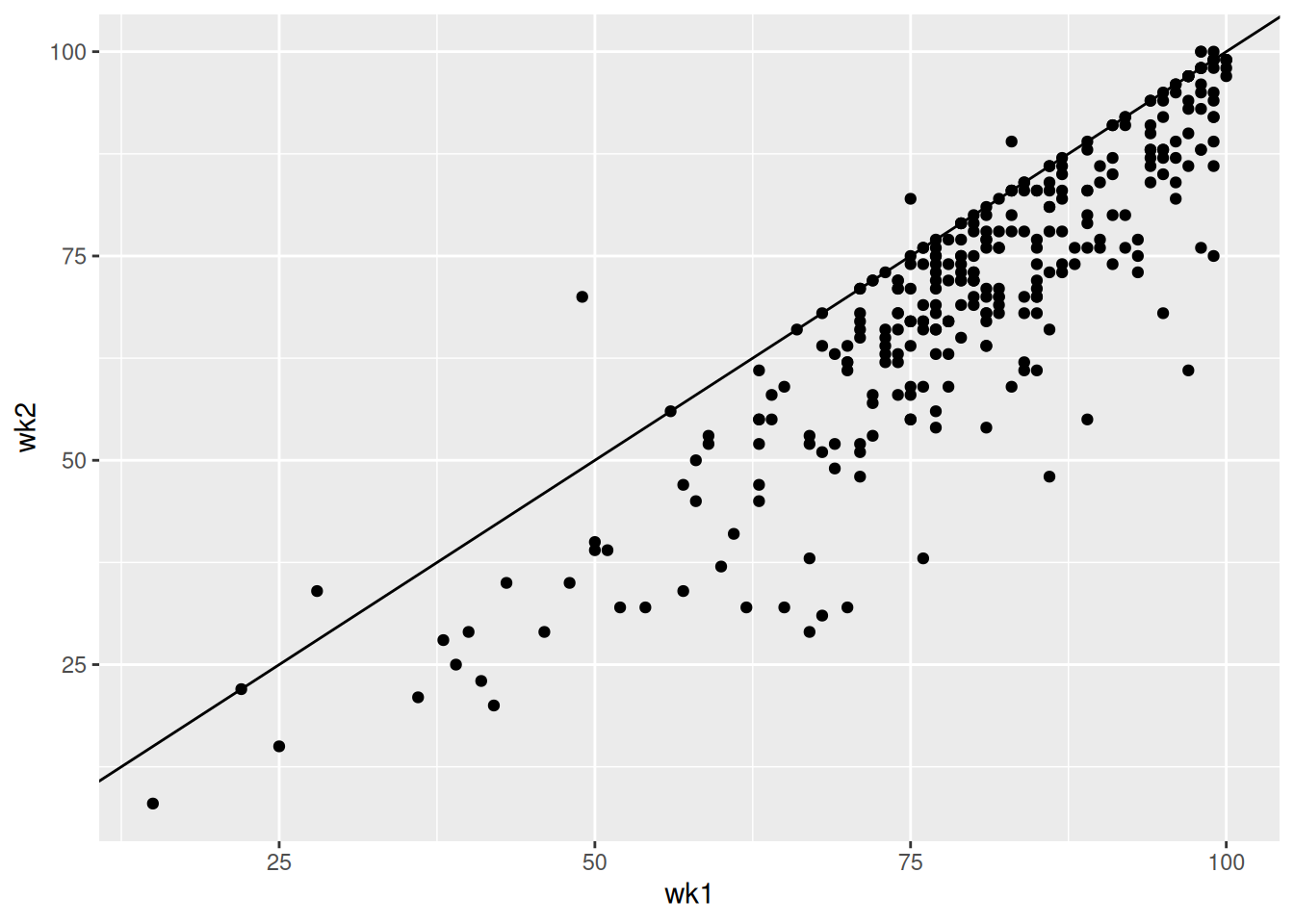
Construct and summarize a plot of how a song’s Billboard ranking its 2nd week on the chart (y-axis) is related to its ranking the 1st week on the charts (x-axis). Add a reference line geom_abline(intercept = 0, slope = 1). Songs above this line improved their rankings from the 1st to 2nd week.

Part b

Use your wrangling tools to identify which songs are those above the line in Part a, i.e. with rankgings that went up from week 1 to week 2.

Part c

Define a new dataset, nov_1999, which:

• only includes data on songs that entered the Billboard charts on November 6, 1999
• keeps all variables except track and date.entered. HINT: How can you avoid writing out all the variable names you want to keep?

# Define nov_1999


# Confirm that nov_1999 has 2 rows (songs) and 77 columns

Part d

Create and discuss a visualization of the rankings (y-axis) over time (x-axis) for the 2 songs in nov_1999. There are hints below (if you scroll), but you’re encouraged to play around and use as few hints as possible.

Hints:

• Should you first pivot wider or longer?
• Once you pivot, the week number is turned into a character variable. How can you change it to a number?

Exercise 6: Practice with the Daily Show

The data associated with this article is available in the fivethirtyeight package, and is loaded into daily below. It includes a list of every guest to ever appear on Jon Stewart’s The Daily Show, a “late-night talk and satirical news” program (per Wikipedia). Check out the dataset and note that when multiple people appeared together, each person receives their own line:

library(fivethirtyeight)
data("daily_show_guests")
daily <- daily_show_guests

In analyzing this data, you’ll need to determine if and when the data needs to be reshaped.

Part a

Identify the 15 guests that appeared the most. (This isn’t a very diverse guest list!)

Part b

CHALLENGE: Create the following data set containing 19 columns:

• The first column should have the 15 guests with the highest number of total appearances on the show, listed in descending order of number of appearances.
• 17 columns should show the number of appearances of the corresponding guest in each year from 1999 to 2015 (one per column).
• Another column should show the total number of appearances for the corresponding guest over the entire duration of the show.

There are hints below (if you scroll), but you’re encouraged to play around and use as few hints as possible.

HINTS: There are lots of ways to do this. You don’t necessarily need all of these hints.

• First obtain the number of times a guest appears each year.
• To this, add a new column which includes the total number of times a guest appears across all years.
• Pivot (longer or wider?). When you do, use values_fill = 0 to replace NA values with 0.
• Arrange, then and keep the top 15.

Part c

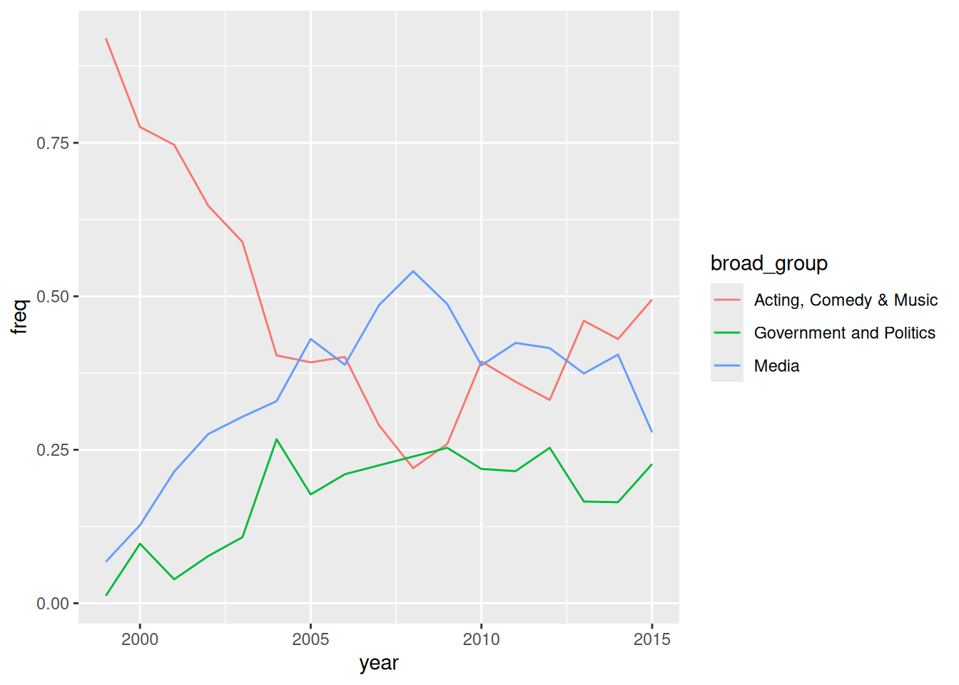
Let’s recreate the first figure from the article. This groups all guests into 3 broader occupational categories. However, our current data has 18 categories:

daily |> 
  count(group)

# A tibble: 18 × 2
   group              n
   <chr>          <int>
 1 Academic         103
 2 Acting           930
 3 Advocacy          24
 4 Athletics         52
 5 Business          25
 6 Clergy             8
 7 Comedy           150
 8 Consultant        18
 9 Government        40
10 Media            751
11 Military          16
12 Misc              45
13 Musician         123
14 Political Aide    36
15 Politician       308
16 Science           28
17 media              5
18 <NA>              31

Let’s define a new dataset that includes a new variable, broad_group, that buckets these 18 categories into the 3 bigger ones used in the article. And get rid of any rows missing information on broad_group. You’ll learn the code soon! For now, just run this chunk:

plot_data <- daily |> 
  mutate(broad_group = case_when(
    group %in% c("Acting", "Athletics", "Comedy", "Musician") ~ "Acting, Comedy & Music",
    group %in% c("Media", "media", "Science", "Academic", "Consultant", "Clergy") ~ "Media",
    group %in% c("Politician", "Political Aide", "Government", "Military", "Business", "Advocacy") ~ "Government and Politics",
    .default = NA
  )) |> 
  filter(!is.na(broad_group))

Now, using the broad_group variable in plot_data, recreate the graphic from the article, with three different lines showing the fraction of guests in each group over time. Note: You’ll have to wrangle the data first.

10.3 Solutions

Click for Solutions

EXAMPLE 1: warm-up counts and proportions

# Using count()
penguins |> 
  count(species, sex)

# A tibble: 8 × 3
  species   sex        n
  <chr>     <chr>  <int>
1 Adelie    female    73
2 Adelie    male      73
3 Adelie    <NA>       6
4 Chinstrap female    34
5 Chinstrap male      34
6 Gentoo    female    58
7 Gentoo    male      61
8 Gentoo    <NA>       5

# Using group_by() and summarize()
penguins |> 
  group_by(species, sex) |> 
  summarize(n())

# A tibble: 8 × 3
# Groups:   species [3]
  species   sex    `n()`
  <chr>     <chr>  <int>
1 Adelie    female    73
2 Adelie    male      73
3 Adelie    <NA>       6
4 Chinstrap female    34
5 Chinstrap male      34
6 Gentoo    female    58
7 Gentoo    male      61
8 Gentoo    <NA>       5

# Relative frequencies
penguins |> 
  group_by(species, sex) |> 
  summarize(n = n()) |> 
  mutate(proportion = n / sum(n))

# A tibble: 8 × 4
# Groups:   species [3]
  species   sex        n proportion
  <chr>     <chr>  <int>      <dbl>
1 Adelie    female    73     0.480 
2 Adelie    male      73     0.480 
3 Adelie    <NA>       6     0.0395
4 Chinstrap female    34     0.5   
5 Chinstrap male      34     0.5   
6 Gentoo    female    58     0.468 
7 Gentoo    male      61     0.492 
8 Gentoo    <NA>       5     0.0403

# Changing the order calculates the proportion of species within each sex
penguins |> 
  group_by(sex, species) |> 
  summarize(n = n()) |> 
  mutate(proportion = n / sum(n))

# A tibble: 8 × 4
# Groups:   sex [3]
  sex    species       n proportion
  <chr>  <chr>     <int>      <dbl>
1 female Adelie       73      0.442
2 female Chinstrap    34      0.206
3 female Gentoo       58      0.352
4 male   Adelie       73      0.435
5 male   Chinstrap    34      0.202
6 male   Gentoo       61      0.363
7 <NA>   Adelie        6      0.545
8 <NA>   Gentoo        5      0.455

EXAMPLE 3: units of observation

# Units of observation = penguins
head(penguins)

# A tibble: 6 × 8
  species island    bill_length_mm bill_depth_mm flipper_length_mm body_mass_g
  <chr>   <chr>              <dbl>         <dbl>             <dbl>       <dbl>
1 Adelie  Torgersen           39.1          18.7               181        3750
2 Adelie  Torgersen           39.5          17.4               186        3800
3 Adelie  Torgersen           40.3          18                 195        3250
4 Adelie  Torgersen           NA            NA                  NA          NA
5 Adelie  Torgersen           36.7          19.3               193        3450
6 Adelie  Torgersen           39.3          20.6               190        3650
# ℹ 2 more variables: sex <chr>, year <dbl>

# Units of observation = species/sex combos
head(penguin_avg)

# A tibble: 6 × 3
# Groups:   species [3]
  species   sex    avg_body_mass
  <chr>     <chr>          <dbl>
1 Adelie    female         3369.
2 Adelie    male           4043.
3 Chinstrap female         3527.
4 Chinstrap male           3939.
5 Gentoo    female         4680.
6 Gentoo    male           5485.

EXAMPLE 5: pivot wider

penguin_avg |> 
  pivot_wider(names_from = sex, values_from = avg_body_mass)

# A tibble: 3 × 3
# Groups:   species [3]
  species   female  male
  <chr>      <dbl> <dbl>
1 Adelie     3369. 4043.
2 Chinstrap  3527. 3939.
3 Gentoo     4680. 5485.

FOLLOW-UP:

• What are the units of observation? species

• Did we lose any information when we widened the data? no

• Use the wide data to calculate the difference in average body mass, male vs female, for each species.

penguin_avg |> 
  pivot_wider(names_from = sex, values_from = avg_body_mass) |> 
  mutate(diff = male - female)

# A tibble: 3 × 4
# Groups:   species [3]
  species   female  male  diff
  <chr>      <dbl> <dbl> <dbl>
1 Adelie     3369. 4043.  675.
2 Chinstrap  3527. 3939.  412.
3 Gentoo     4680. 5485.  805.

EXAMPLE 6: Pivot longer

# We can either communicate which variables we WANT to collect into a single column (female, male)
penguin_avg_wide |> 
  pivot_longer(cols = c(female, male), names_to = "sex", values_to = "avg_body_mass")

# A tibble: 6 × 3
# Groups:   species [3]
  species   sex    avg_body_mass
  <chr>     <chr>          <dbl>
1 Adelie    female         3369.
2 Adelie    male           4043.
3 Chinstrap female         3527.
4 Chinstrap male           3939.
5 Gentoo    female         4680.
6 Gentoo    male           5485.

# Or which variable(s) we do NOT want to collect into a single column (sex)
penguin_avg_wide |> 
  pivot_longer(cols = -species, names_to = "sex", values_to = "avg_body_mass")

# A tibble: 6 × 3
# Groups:   species [3]
  species   sex    avg_body_mass
  <chr>     <chr>          <dbl>
1 Adelie    female         3369.
2 Adelie    male           4043.
3 Chinstrap female         3527.
4 Chinstrap male           3939.
5 Gentoo    female         4680.
6 Gentoo    male           5485.

FOLLOW-UP:

• What are the units of observation? species/sex combos

• Did we lose any information when we lengthened the data? no

EXAMPLE 7: Practice

food <- data.frame(
  customer = rep(c("A", "B"), each = 3),
  restaurant = rep(c("Shish", "FrenchMeadow", "DunnBros"), 2),
  order = c("falafel", "salad", "coffee", "baklava", "pastry", "tea")
)

food

  customer   restaurant   order
1        A        Shish falafel
2        A FrenchMeadow   salad
3        A     DunnBros  coffee
4        B        Shish baklava
5        B FrenchMeadow  pastry
6        B     DunnBros     tea

food |> 
  pivot_wider(names_from = restaurant, values_from = order)

# A tibble: 2 × 4
  customer Shish   FrenchMeadow DunnBros
  <chr>    <chr>   <chr>        <chr>   
1 A        falafel salad        coffee  
2 B        baklava pastry       tea     

more_food <- data.frame(
  customer = c("C", "D"),
  Shish = c("coffee", "maza"),
  FrenchMeadow = c("soup", "sandwich"),
  DunnBros = c("cookie", "coffee")
)

more_food

  customer  Shish FrenchMeadow DunnBros
1        C coffee         soup   cookie
2        D   maza     sandwich   coffee

more_food |> 
  pivot_longer(cols = -customer, names_to = "restaurant", values_to = "order")

# A tibble: 6 × 3
  customer restaurant   order   
  <chr>    <chr>        <chr>   
1 C        Shish        coffee  
2 C        FrenchMeadow soup    
3 C        DunnBros     cookie  
4 D        Shish        maza    
5 D        FrenchMeadow sandwich
6 D        DunnBros     coffee  

Exercise 1: What’s the problem?

Part a

subjects/people

Part c

pivot_longer()

Exercise 2: Pivot longer

Part a

# For cols, try 2 appproaches: using - and starts_with
sleep_wide |>
  pivot_longer(cols = -Subject, names_to = "day", values_to = "reaction_time")

# A tibble: 180 × 3
   Subject day   reaction_time
     <int> <chr>         <dbl>
 1     308 day_0          250.
 2     308 day_1          259.
 3     308 day_2          251.
 4     308 day_3          321.
 5     308 day_4          357.
 6     308 day_5          415.
 7     308 day_6          382.
 8     308 day_7          290.
 9     308 day_8          431.
10     308 day_9          466.
# ℹ 170 more rows

sleep_wide |>
  pivot_longer(cols = starts_with("day"), names_to = "day", values_to = "reaction_time")

# A tibble: 180 × 3
   Subject day   reaction_time
     <int> <chr>         <dbl>
 1     308 day_0          250.
 2     308 day_1          259.
 3     308 day_2          251.
 4     308 day_3          321.
 5     308 day_4          357.
 6     308 day_5          415.
 7     308 day_6          382.
 8     308 day_7          290.
 9     308 day_8          431.
10     308 day_9          466.
# ℹ 170 more rows

Part b

Adding names_prefix = "day_" removed “day_” from the start of the day entries. did this impact how the values are recorded in the day column?

sleep_long <- sleep_wide |>
  pivot_longer(cols = -Subject,
               names_to = "day",
               names_prefix = "day_",
               values_to = "reaction_time") 

Part c

Subject is an integer and day is a character. We want them to be categorical (factor) and numeric, respectively.

ggplot(sleep_long, aes(y = reaction_time, x = day, color = Subject)) + 
  geom_line()

Exercise 3: Changing variable classes & plotting

sleep_long <- sleep_wide |>
  pivot_longer(cols = -Subject,
               names_to = "day",
               names_prefix = "day_",
               values_to = "reaction_time") |> 
  mutate(Subject = as.factor(Subject), day = as.numeric(day))

Part a

Now make some plots.

# Make a line plot of reaction time by day for each subject
# Put these all on the same frame
ggplot(sleep_long, aes(y = reaction_time, x = day, color = Subject)) + 
  geom_line()

# Make a line plot of reaction time by day for each subject
# Put these all on separate frames (one per subject)
ggplot(sleep_long, aes(y = reaction_time, x = day, color = Subject)) + 
  geom_line() + 
  facet_wrap(~ Subject)

Part b

Reaction time increases (worsens) with a lack of sleep. Some subjects seem to be more impacted than others by lack of sleep, and some tend to have faster/slower reaction times in general.

Exercise 4: Pivot wider

Part a

sleep_long |>
  pivot_wider(names_from = day, values_from = reaction_time) |>
  head()

# A tibble: 6 × 11
  Subject   `0`   `1`   `2`   `3`   `4`   `5`   `6`   `7`   `8`   `9`
  <fct>   <dbl> <dbl> <dbl> <dbl> <dbl> <dbl> <dbl> <dbl> <dbl> <dbl>
1 308      250.  259.  251.  321.  357.  415.  382.  290.  431.  466.
2 309      223.  205.  203.  205.  208.  216.  214.  218.  224.  237.
3 310      199.  194.  234.  233.  229.  220.  235.  256.  261.  248.
4 330      322.  300.  284.  285.  286.  298.  280.  318.  305.  354.
5 331      288.  285   302.  320.  316.  293.  290.  335.  294.  372.
6 332      235.  243.  273.  310.  317.  310   454.  347.  330.  254.

Part b

sleep_long |>
  pivot_wider(names_from = day, values_from = reaction_time, names_prefix = "day_") |>
  head()

# A tibble: 6 × 11
  Subject day_0 day_1 day_2 day_3 day_4 day_5 day_6 day_7 day_8 day_9
  <fct>   <dbl> <dbl> <dbl> <dbl> <dbl> <dbl> <dbl> <dbl> <dbl> <dbl>
1 308      250.  259.  251.  321.  357.  415.  382.  290.  431.  466.
2 309      223.  205.  203.  205.  208.  216.  214.  218.  224.  237.
3 310      199.  194.  234.  233.  229.  220.  235.  256.  261.  248.
4 330      322.  300.  284.  285.  286.  298.  280.  318.  305.  354.
5 331      288.  285   302.  320.  316.  293.  290.  335.  294.  372.
6 332      235.  243.  273.  310.  317.  310   454.  347.  330.  254.

Exercise 5: Practice with Billboard charts

Part a

The higher a song’s week 1 rating, the higher its week 2 rating tends to be. But almost all song’s rankings drop from week 1 to week 2.

ggplot(billboard, aes(y = wk2, x = wk1)) + 
  geom_point() +
  geom_abline(intercept = 0, slope = 1)

Part b

billboard |> 
  filter(wk2 > wk1)

# A tibble: 7 × 79
  artist      track date.entered   wk1   wk2   wk3   wk4   wk5   wk6   wk7   wk8
  <chr>       <chr> <date>       <dbl> <dbl> <dbl> <dbl> <dbl> <dbl> <dbl> <dbl>
1 Carey, Mar… Cryb… 2000-06-24      28    34    48    62    77    90    95    NA
2 Clark, Ter… A Li… 2000-12-16      75    82    88    96    99    99    NA    NA
3 Diffie, Joe The … 2000-01-01      98   100   100    90    93    94    NA    NA
4 Hart, Beth  L.A.… 1999-11-27      99   100    98    99    99    99    98    90
5 Jay-Z       Hey … 2000-08-12      98   100    98    94    83    83    80    78
6 Lil' Zane   Call… 2000-07-29      83    89    57    40    34    21    33    46
7 Pearl Jam   Noth… 2000-05-13      49    70    84    89    93    91    NA    NA
# ℹ 68 more variables: wk9 <dbl>, wk10 <dbl>, wk11 <dbl>, wk12 <dbl>,
#   wk13 <dbl>, wk14 <dbl>, wk15 <dbl>, wk16 <dbl>, wk17 <dbl>, wk18 <dbl>,
#   wk19 <dbl>, wk20 <dbl>, wk21 <dbl>, wk22 <dbl>, wk23 <dbl>, wk24 <dbl>,
#   wk25 <dbl>, wk26 <dbl>, wk27 <dbl>, wk28 <dbl>, wk29 <dbl>, wk30 <dbl>,
#   wk31 <dbl>, wk32 <dbl>, wk33 <dbl>, wk34 <dbl>, wk35 <dbl>, wk36 <dbl>,
#   wk37 <dbl>, wk38 <dbl>, wk39 <dbl>, wk40 <dbl>, wk41 <dbl>, wk42 <dbl>,
#   wk43 <dbl>, wk44 <dbl>, wk45 <dbl>, wk46 <dbl>, wk47 <dbl>, wk48 <dbl>, …

Part c

# Define nov_1999
nov_1999 <- billboard |> 
  filter(date.entered == "1999-11-06") |> 
  select(-track, -date.entered)

# Or
nov_1999 <- billboard |> 
  filter(date.entered == "1999-11-06") |> 
  select(artist, starts_with("wk"))


# Confirm that nov_1999 has 2 rows (songs) and 77 columns
dim(nov_1999)

[1]  2 77

Part c

nov_1999 |> 
  pivot_longer(cols = -artist, names_to = "week", names_prefix = "wk", values_to = "ranking") |> 
  mutate(week = as.numeric(week)) |> 
  ggplot(aes(y = ranking, x = week, color = artist)) + 
    geom_line()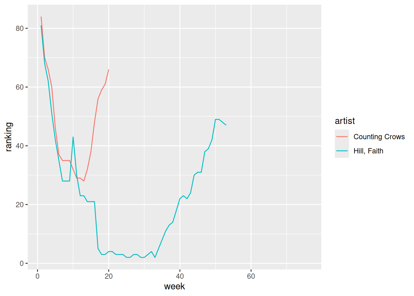

Exercise 6: Practice with the Daily Show

Part a

daily |> 
  count(raw_guest_list) |> 
  arrange(desc(n)) |> 
  head(15)

# A tibble: 15 × 2
   raw_guest_list        n
   <chr>             <int>
 1 Fareed Zakaria       19
 2 Denis Leary          17
 3 Brian Williams       16
 4 Paul Rudd            13
 5 Ricky Gervais        13
 6 Tom Brokaw           12
 7 Bill O'Reilly        10
 8 Reza Aslan           10
 9 Richard Lewis        10
10 Will Ferrell         10
11 Sarah Vowell          9
12 Adam Sandler          8
13 Ben Affleck           8
14 Louis C.K.            8
15 Maggie Gyllenhaal     8

Part b

daily |> 
  count(year, raw_guest_list) |> 
  group_by(raw_guest_list) |> 
  mutate(total = sum(n)) |>
  pivot_wider(names_from = year, 
              values_from = n,
              values_fill = 0) |> 
  arrange(desc(total)) |> 
  head(15)

# A tibble: 15 × 19
# Groups:   raw_guest_list [15]
   raw_guest_list  total `1999` `2000` `2001` `2002` `2003` `2004` `2005` `2006`
   <chr>           <int>  <int>  <int>  <int>  <int>  <int>  <int>  <int>  <int>
 1 Fareed Zakaria     19      0      0      1      0      1      2      2      2
 2 Denis Leary        17      1      0      1      2      1      0      0      1
 3 Brian Williams     16      0      0      0      0      1      1      2      1
 4 Paul Rudd          13      1      0      1      1      1      1      1      0
 5 Ricky Gervais      13      0      0      0      0      0      0      1      2
 6 Tom Brokaw         12      0      0      0      1      0      2      1      0
 7 Richard Lewis      10      1      0      2      2      1      1      0      0
 8 Will Ferrell       10      0      1      1      0      1      1      1      1
 9 Bill O'Reilly      10      0      0      1      1      0      1      1      0
10 Reza Aslan         10      0      0      0      0      0      0      1      2
11 Sarah Vowell        9      0      0      0      1      0      1      1      1
12 Adam Sandler        8      1      2      0      1      0      0      0      1
13 Ben Affleck         8      0      0      0      0      2      0      0      1
14 Maggie Gyllenh…     8      0      0      0      0      1      0      1      1
15 Louis C.K.          8      0      0      0      0      0      0      0      1
# ℹ 9 more variables: `2007` <int>, `2008` <int>, `2009` <int>, `2010` <int>,
#   `2011` <int>, `2012` <int>, `2013` <int>, `2014` <int>, `2015` <int>

Part c

plot_data |>
  group_by(year, broad_group) |>
  summarise(n = n()) |>
  mutate(freq = n / sum(n)) |> 
  ggplot(aes(y = freq, x = year, color = broad_group)) + 
    geom_line()

---

1. Gregory Belenky, Nancy J. Wesensten, David R. Thorne, Maria L. Thomas, Helen C. Sing, Daniel P. Redmond, Michael B. Russo and Thomas J. Balkin (2003) Patterns of performance degradation and restoration during sleep restriction and subsequent recovery: a sleep dose-response study. Journal of Sleep Research 12, 1–12.