13  Strings

Learning Goals

• Learn some fundamentals of working with strings of text data.
• Learn functions to search and replace, detect patterns, locate patterns, extract patterns, and separate text with the stringr package.

Additional Resources

For more information about the topics covered in this chapter, refer to the resources below:

• Working with strings (YouTube) by Lisa Lendway
• strings cheat sheet (pdf)
• Strings (html) by Wickham, Çetinkaya-Rundel, & Grolemund
• Regular expressions (html) by Baumer, Kaplan, and Horton
• RegExplain RStudio addin tool (html) (Garrick Aden-Buie)
• regexr exploration tool (html)

Instructions

General

• Be kind to yourself.
• Collaborate with and be kind to others. You are expected to work together as a group.
• Ask questions. Remember that we won’t discuss these exercises as a class.

Activity Specific

Help each other with the following:

• Create a new Quarto document in the activities folder of your portfolio project and do not forgot to include it in _quarto.yml file. Then click the </> Code link at the top right corner of this page and copy the code into the created Quarto document. This is where you’ll take notes. Remember that the portfolio is yours, so take notes in whatever way is best for you.
• Don’t start the Exercises section before we get there as a class. First, engage in class discussion and eventually collaborate with your group on the exercises!

13.1 Warm-up

WHERE ARE WE?

We’re in the last day of our “data preparation” unit:

In the previous class, we started discussing some considerations in working with special types of “categorical” variables: characters and factors which are:

1. Converting characters to factors (and factors to meaningful factors)–last time
   When categorical information is stored as a character variable, the categories of interest might not be labeled or ordered in a meaningful way. We can fix that!

2. Strings–today!
   When working with character strings, we might want to detect, replace, or extract certain patterns. For example, recall our data on courses:

    sessionID dept level    sem enroll     iid
1 session1784    M   100 FA1991     22 inst265
2 session1785    k   100 FA1991     52 inst458
3 session1791    J   100 FA1993     22 inst223
4 session1792    J   300 FA1993     20 inst235
5 session1794    J   200 FA1993     22 inst234
6 session1795    J   200 SP1994     26 inst230

'data.frame':   1718 obs. of  6 variables:
 $ sessionID: chr  "session1784" "session1785" "session1791" "session1792" ...
 $ dept     : chr  "M" "k" "J" "J" ...
 $ level    : int  100 100 100 300 200 200 200 100 300 100 ...
 $ sem      : chr  "FA1991" "FA1991" "FA1993" "FA1993" ...
 $ enroll   : int  22 52 22 20 22 26 25 38 16 43 ...
 $ iid      : chr  "inst265" "inst458" "inst223" "inst235" ...

Focusing on just the sem character variable, we might want to…

• change FA to fall_ and SP to spring_
• keep only courses taught in fall
• split the variable into 2 new variables: semester (FA or SP) and year

3. Much more!–maybe in your projects or COMP/STAT 212
   There are a lot of ways to process character variables. For example, we might have a variable that records the text for a sample of news articles. We might want to analyze things like the articles’ sentiments, word counts, typical word lengths, most common words, etc.

ESSENTIAL STRING FUNCTIONS

The stringr package within tidyverse contains lots of functions to help process strings. We’ll focus on the most common. Letting x be a string variable…

function	arguments	returns
str_replace()	x, pattern, replacement	a modified string
str_replace_all()	x, pattern, replacement	a modified string
str_to_lower()	x	a modified string
str_sub()	x, start, end	a modified string
str_length()	x	a number
str_detect()	x, pattern	TRUE/FALSE

EXAMPLE 1

Consider the following data with string variables :

library(tidyverse)

classes <- data.frame(
  sem        = c("SP2023", "FA2023", "SP2024"),
  area       = c("History", "Math", "Anthro"),
  enroll     = c("30 - people", "20 - people", "25 - people"),
  instructor = c("Ernesto Capello", "Lori Ziegelmeier", "Arjun Guneratne")
)

classes

     sem    area      enroll       instructor
1 SP2023 History 30 - people  Ernesto Capello
2 FA2023    Math 20 - people Lori Ziegelmeier
3 SP2024  Anthro 25 - people  Arjun Guneratne

Using only your intuition, use our str_ functions to complete the following. NOTE: You might be able to use other wrangling verbs in some cases, but focus on the new functions here.

# Define a new variable "num" that adds up the number of characters in the area label

# Change the areas to "history", "math", "anthro" instead of "History", "Math", "Anthro"

# Create a variable that id's which courses were taught in spring

# Change the semester labels to "fall2023", "spring2024", "spring2023"

# In the enroll variable, change all e's to 3's (just because?)

# Use sem to create 2 new variables, one with only the semester (SP/FA) and 1 with the year

SUMMARY

Here’s what we learned about each function:

• str_replace(x, pattern, replacement) finds the first part of x that matches the pattern and replaces it with replacement

• str_replace_all(x, pattern, replacement) finds all instances in x that matches the pattern and replaces it with replacement

• str_to_lower(x) converts all upper case letters in x to lower case

• str_sub(x, start, end) only keeps a subset of characters in x, from start (a number indexing the first letter to keep) to end (a number indexing the last letter to keep)

• str_length(x) records the number of characters in x

• str_detect(x, pattern) is TRUE if x contains the given pattern and FALSE otherwise

EXAMPLE 2

Suppose we only want the spring courses:

# How can we do this after mutating?
classes |> 
  mutate(spring = str_detect(sem, "SP"))

     sem    area      enroll       instructor spring
1 SP2023 History 30 - people  Ernesto Capello   TRUE
2 FA2023    Math 20 - people Lori Ziegelmeier  FALSE
3 SP2024  Anthro 25 - people  Arjun Guneratne   TRUE

# We don't have to mutate first!
classes |> 
  filter(str_detect(sem, "SP"))

     sem    area      enroll      instructor
1 SP2023 History 30 - people Ernesto Capello
2 SP2024  Anthro 25 - people Arjun Guneratne

# Yet another way
classes |> 
  filter(!str_detect(sem, "FA"))

     sem    area      enroll      instructor
1 SP2023 History 30 - people Ernesto Capello
2 SP2024  Anthro 25 - people Arjun Guneratne

EXAMPLE 3

Suppose we wanted to get separate columns for the first and last names of each course instructor in classes. Try doing this using str_sub(). But don’t try too long! Explain what trouble you ran into.

EXAMPLE 4

In general, when we want to split a column into 2+ new columns, we can often use separate():

classes |> 
  separate(instructor, c("first", "last"), sep = " ")

     sem    area      enroll   first        last
1 SP2023 History 30 - people Ernesto     Capello
2 FA2023    Math 20 - people    Lori Ziegelmeier
3 SP2024  Anthro 25 - people   Arjun   Guneratne

# Sometimes the function can "intuit" how we want to separate the variable
classes |> 
  separate(instructor, c("first", "last"))

     sem    area      enroll   first        last
1 SP2023 History 30 - people Ernesto     Capello
2 FA2023    Math 20 - people    Lori Ziegelmeier
3 SP2024  Anthro 25 - people   Arjun   Guneratne

1. Separate enroll into 2 separate columns: students and people. (These columns don’t make sense this is just practice).

# classes |> 
#   separate(___, c(___, ___), sep = "___")

2. We separated sem into semester and year above using str_sub(). Why would this be hard using separate()?

3. When we want to split a column into 2+ new columns (or do other types of string processing), but there’s no consistent pattern by which to do this, we can use regular expressions (an optional topic):

# (?<=[SP|FA]): any character *before* the split point is a "SP" or "FA"
# (?=2): the first character *after* the split point is a 2
classes |> 
  separate(sem, 
          c("semester", "year"),
          "(?<=[SP|FA])(?=2)")

  semester year    area      enroll       instructor
1       SP 2023 History 30 - people  Ernesto Capello
2       FA 2023    Math 20 - people Lori Ziegelmeier
3       SP 2024  Anthro 25 - people  Arjun Guneratne

# More general:
# (?<=[a-zA-Z]): any character *before* the split point is a lower or upper case letter
# (?=[0-9]): the first character *after* the split point is number
classes |> 
  separate(sem, 
          c("semester", "year"),
          "(?<=[A-Z])(?=[0-9])")

  semester year    area      enroll       instructor
1       SP 2023 History 30 - people  Ernesto Capello
2       FA 2023    Math 20 - people Lori Ziegelmeier
3       SP 2024  Anthro 25 - people  Arjun Guneratne

13.2 Exercises

Exercise 1: Time slots

The courses data includes actual data scraped from Mac’s class schedule. (Thanks to Prof Leslie Myint for the scraping code!!)

If you want to learn how to scrape data, take COMP/STAT 212, Intermediate Data Science! NOTE: For simplicity, I removed classes that had “TBA” for the days.

courses <- read.csv("https://mac-stat.github.io/data/registrar.csv")

# Check it out
head(courses)

       number   crn                                                name  days
1 AMST 112-01 10318         Introduction to African American Literature M W F
2 AMST 194-01 10073              Introduction to Asian American Studies M W F
3 AMST 194-F1 10072 What’s After White Empire - And Is It Already Here?  T R 
4 AMST 203-01 10646 Politics and Inequality: The American Welfare State M W F
5 AMST 205-01 10842                         Trans Theories and Politics  T R 
6 AMST 209-01 10474                   Civil Rights in the United States   W  
             time      room             instructor avail_max
1 9:40 - 10:40 am  MAIN 009       Daylanne English    3 / 20
2  1:10 - 2:10 pm MUSIC 219          Jake Nagasawa   -4 / 16
3  3:00 - 4:30 pm   HUM 214 Karin Aguilar-San Juan    0 / 14
4 9:40 - 10:40 am  CARN 305          Lesley Lavery    3 / 25
5  3:00 - 4:30 pm  MAIN 009              Myrl Beam   -2 / 20
6 7:00 - 10:00 pm  MAIN 010         Walter Greason   -1 / 15

Use our more familiar wrangling tools to warm up.

# Construct a table that indicates the number of classes offered in each day/time slot
# Print only the 6 most popular time slots

Exercise 2: Prep the data

So that we can analyze it later, we want to wrangle the courses data:

• Let’s get some enrollment info:
  • Split avail_max into 2 separate variables: avail and max.
  • Use avail and max to define a new variable called enrollment. HINT: You’ll need as.numeric()
• Split the course number into 3 separate variables: dept, number, and section. HINT: You can use separate() to split a variable into 3, not just 2 new variables.

Store this as courses_clean so that you can use it later.

Exercise 3: Courses by department

Using courses_clean…

# Identify the 6 departments that offered the most sections


# Identify the 6 departments with the longest average course titles

Exercise 4: STAT courses

Part a

Get a subset of courses_clean that only includes courses taught by Alicia Johnson.

Part b

Create a new dataset from courses_clean, named stat, that only includes STAT sections. In this dataset:

• In the course names:

  • Remove “Introduction to” from any name.
  • Shorten “Statistical” to “Stat” where relevant.

• Define a variable that records the start_time for the course.

• Keep only the number, name, start_time, enroll columns.

• The result should have 18 rows and 4 columns.

Exercise 5: More cleaning

In the next exercises, we’ll dig into enrollments. Let’s get the data ready for that analysis here. Make the following changes to the courses_clean data. Because they have different enrollment structures, and we don’t want to compare apples and oranges, remove the following:

• all sections in PE and INTD (interdisciplinary studies courses)

• all music ensembles and dance practicums, i.e. all MUSI and THDA classes with numbers less than 100. HINT: !(dept == "MUSI" & as.numeric(number) < 100)

• all lab sections. Be careful which variable you use here. For example, you don’t want to search by “Lab” and accidentally eliminate courses with words such as “Labor”.

Save the results as enrollments (don’t overwrite courses_clean).

Exercise 6: Enrollment & departments

Explore enrollments by department. You decide what research questions to focus on. Use both visual and numerical summaries.

Exercise 7: Enrollment & faculty

Let’s now explore enrollments by instructor. In doing so, we have to be cautious of cross-listed courses that are listed under multiple different departments. Uncomment the code lines in the chunk below for an example.

Commenting/Uncommenting Code

To comment/uncomment several lines of code at once, highlight them then click ctrl/cmd+shift+c.

# enrollments |>
#   filter(dept %in% c("STAT", "COMP"), number == 112, section == "01")

Notice that these are the exact same section! In order to not double count an instructor’s enrollments, we can keep only the courses that have distinct() combinations of days, time, instructor values. Uncomment the code lines in the chunk below.

# enrollments_2 <- enrollments |> 
#   distinct(days, time, instructor, .keep_all = TRUE)

# NOTE: By default this keeps the first department alphabetically
# That's fine because we won't use this to analyze department enrollments!
# enrollments_2 |> 
#   filter(instructor == "Brianna Heggeseth", name == "Introduction to Data Science")

Now, explore enrollments by instructor. You decide what research questions to focus on. Use both visual and numerical summaries.

CAVEAT: The above code doesn’t deal with co-taught courses that have more than one instructor. Thus instructors that co-taught are recorded as a pair, and their co-taught enrollments aren’t added to their total enrollments. This is tough to get around with how the data were scraped as the instructor names are smushed together, not separated by a comma!

Optional extra practice

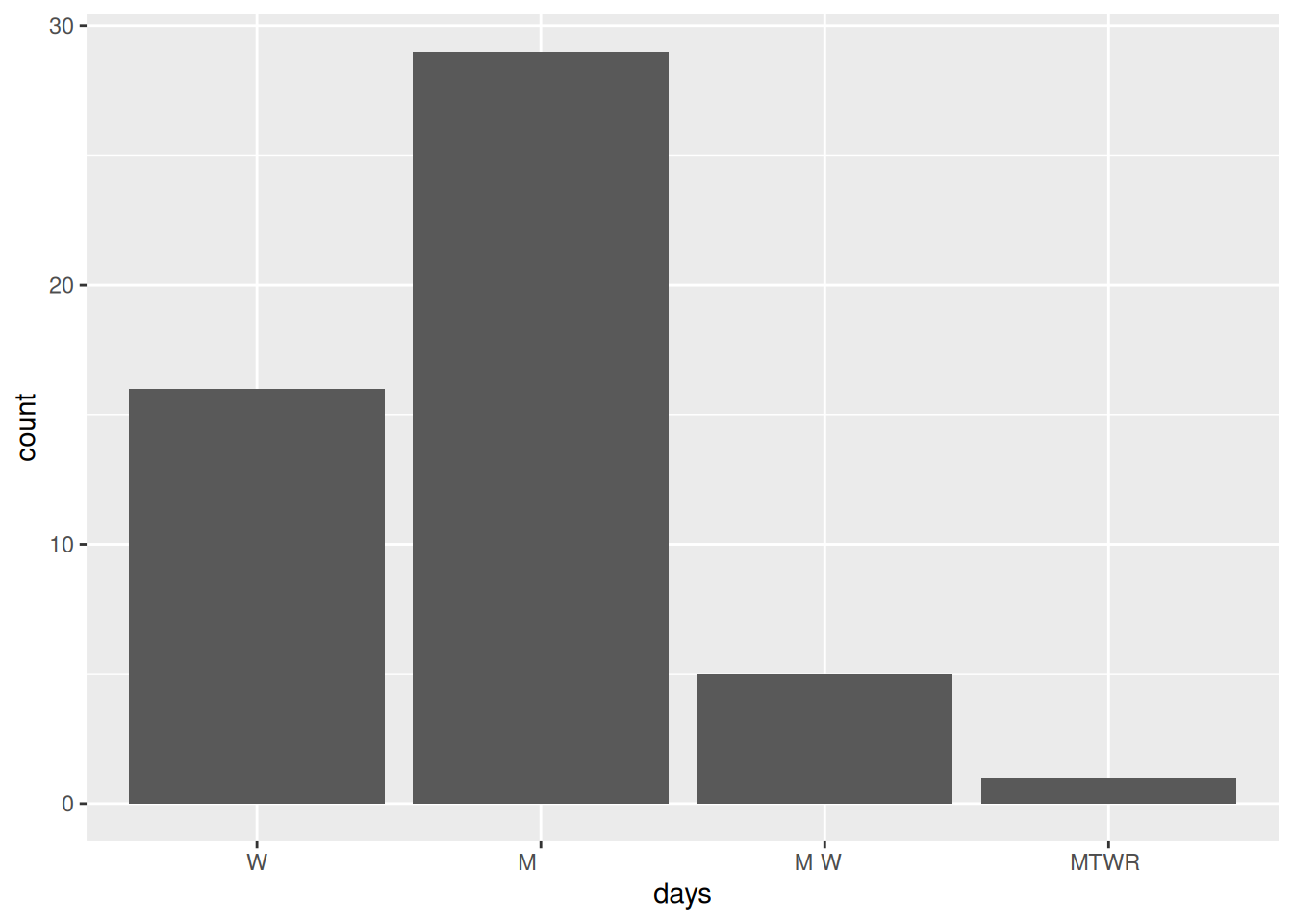
# Make a bar plot showing the number of night courses by day of the week
# Use courses_clean

Dig Deeper: regex

Example 4 gave 1 small example of a regular expression.

These are handy when we want process a string variable, but there’s no consistent pattern by which to do this. You must think about the structure of the string and how you can use regular expressions to capture the patterns you want (and exclude the patterns you don’t want).

For example, how would you describe the pattern of a 10-digit phone number? Limit yourself to just a US phone number for now.

• The first 3 digits are the area code.
• The next 3 digits are the exchange code.
• The last 4 digits are the subscriber number.

Thus, a regular expression for a US phone number could be:

• [:digit:]{3}-[:digit:]{3}-[:digit:]{4} which limits you to XXX-XXX-XXXX pattern or
• \\([:digit:]{3}\\) [:digit:]{3}-[:digit:]{4} which limits you to (XXX) XXX-XXXX pattern or
• [:digit:]{3}\\.[:digit:]{3}\\.[:digit:]{4} which limits you to XXX.XXX.XXXX pattern

The following would include the three patterns above in addition to the XXXXXXXXXX pattern (no dashes or periods): - [\\(]*[:digit:]{3}[-.\\)]*[:digit:]{3}[-.]*[:digit:]{4}

In order to write a regular expression, you first need to consider what patterns you want to include and exclude.

Work through the following examples, and the tutorial after them to learn about the syntax.

EXAMPLES

# Define some strings to play around with
example <- "The quick brown fox jumps over the lazy dog."

str_replace(example, "quick", "really quick")

[1] "The really quick brown fox jumps over the lazy dog."

str_replace_all(example, "(fox|dog)", "****") # | reads as OR

[1] "The quick brown **** jumps over the lazy ****."

str_replace_all(example, "(fox|dog).", "****") # "." for any character

[1] "The quick brown ****jumps over the lazy ****"

str_replace_all(example, "(fox|dog)\\.$", "****") # at end of sentence only, "\\." only for a period

[1] "The quick brown fox jumps over the lazy ****"

str_replace_all(example, "the", "a") # case-sensitive only matches one

[1] "The quick brown fox jumps over a lazy dog."

str_replace_all(example, "[Tt]he", "a") # # will match either t or T; could also make "a" conditional on capitalization of t

[1] "a quick brown fox jumps over a lazy dog."

str_replace_all(example, "[Tt]he", "a") # first match only

[1] "a quick brown fox jumps over a lazy dog."

# More examples
example2 <- "Two roads diverged in a yellow wood, / And sorry I could not travel both / And be one traveler, long I stood / And looked down one as far as I could"
example3 <- "This is a test"

# Store the examples in 1 place
examples <- c(example, example2, example3)

pat <- "[^aeiouAEIOU ]{3}" # Regular expression for three straight consonants. Note that I've excluded spaces as well

str_detect(examples, pat) # TRUE/FALSE if it detects pattern

[1]  TRUE  TRUE FALSE

str_subset(examples, pat) # Pulls out those that detects pattern

[1] "The quick brown fox jumps over the lazy dog."                                                                                                        
[2] "Two roads diverged in a yellow wood, / And sorry I could not travel both / And be one traveler, long I stood / And looked down one as far as I could"

pat2 <- "[^aeiouAEIOU ][aeiouAEIOU]{2}[^aeiouAEIOU ]{1}" # consonant followed by two vowels followed by a consonant

str_extract(example2, pat2) # extract first match

[1] "road"

str_extract_all(example2, pat2, simplify = TRUE) # extract all matches

     [,1]   [,2]   [,3]   [,4]   [,5]   [,6]  
[1,] "road" "wood" "coul" "tood" "look" "coul"

TUTORIAL

Try out this interactive tutorial. Note that neither the tutorial nor regular expressions more generally are specific to R, but it still illustrates the main ideas of regular expressions.

13.3 Solutions

Click for Solutions

EXAMPLE 1

# Define a new variable "num" that adds up the number of characters in the area label
classes |> 
  mutate(num = str_length(area))

     sem    area      enroll       instructor num
1 SP2023 History 30 - people  Ernesto Capello   7
2 FA2023    Math 20 - people Lori Ziegelmeier   4
3 SP2024  Anthro 25 - people  Arjun Guneratne   6

# Change the areas to "history", "math", "anthro"
classes |> 
  mutate(area = str_to_lower(area))

     sem    area      enroll       instructor
1 SP2023 history 30 - people  Ernesto Capello
2 FA2023    math 20 - people Lori Ziegelmeier
3 SP2024  anthro 25 - people  Arjun Guneratne

# Create a variable that id's which courses were taught in spring 
classes |> 
  mutate(spring = str_detect(sem, "SP"))

     sem    area      enroll       instructor spring
1 SP2023 History 30 - people  Ernesto Capello   TRUE
2 FA2023    Math 20 - people Lori Ziegelmeier  FALSE
3 SP2024  Anthro 25 - people  Arjun Guneratne   TRUE

# Change the semester labels to "fall2023", "spring2024", "spring2023"
classes |> 
  mutate(sem = str_replace(sem, "SP", "spring")) |> 
  mutate(sem = str_replace(sem, "FA", "fall"))

         sem    area      enroll       instructor
1 spring2023 History 30 - people  Ernesto Capello
2   fall2023    Math 20 - people Lori Ziegelmeier
3 spring2024  Anthro 25 - people  Arjun Guneratne

# In the enroll variable, change all e's to 3's (just because?)
classes |> 
  mutate(enroll = str_replace_all(enroll, "e", "3"))

     sem    area      enroll       instructor
1 SP2023 History 30 - p3opl3  Ernesto Capello
2 FA2023    Math 20 - p3opl3 Lori Ziegelmeier
3 SP2024  Anthro 25 - p3opl3  Arjun Guneratne

# Use sem to create 2 new variables, one with only the semester (SP/FA) and 1 with the year
classes |> 
  mutate(semester = str_sub(sem, 1, 2),
         year = str_sub(sem, 3, 6))

     sem    area      enroll       instructor semester year
1 SP2023 History 30 - people  Ernesto Capello       SP 2023
2 FA2023    Math 20 - people Lori Ziegelmeier       FA 2023
3 SP2024  Anthro 25 - people  Arjun Guneratne       SP 2024

EXAMPLE 2

# How can we do this after mutating?
classes |> 
  mutate(spring = str_detect(sem, "SP")) |> 
  filter(spring == TRUE)

     sem    area      enroll      instructor spring
1 SP2023 History 30 - people Ernesto Capello   TRUE
2 SP2024  Anthro 25 - people Arjun Guneratne   TRUE

Exercise 1: Popular time slots

# Construct a table that indicates the number of classes offered in each day/time slot
# Print only the 6 most popular time slots
courses |> 
  count(days, time) |> 
  arrange(desc(n)) |> 
  head()

   days             time  n
1 M W F 10:50 - 11:50 am 76
2  T R   9:40 - 11:10 am 71
3 M W F  9:40 - 10:40 am 68
4 M W F   1:10 - 2:10 pm 66
5  T R    3:00 - 4:30 pm 62
6  T R    1:20 - 2:50 pm 59

Exercise 2: Prep the data

courses_clean <- courses |> 
  separate(avail_max, c("avail", "max"), sep = " / ") |> 
  mutate(enroll = as.numeric(max) - as.numeric(avail)) |> 
  separate(number, c("dept", "number", "section"))
  
head(courses_clean)

  dept number section   crn                                                name
1 AMST    112      01 10318         Introduction to African American Literature
2 AMST    194      01 10073              Introduction to Asian American Studies
3 AMST    194      F1 10072 What’s After White Empire - And Is It Already Here?
4 AMST    203      01 10646 Politics and Inequality: The American Welfare State
5 AMST    205      01 10842                         Trans Theories and Politics
6 AMST    209      01 10474                   Civil Rights in the United States
   days            time      room             instructor avail max enroll
1 M W F 9:40 - 10:40 am  MAIN 009       Daylanne English     3  20     17
2 M W F  1:10 - 2:10 pm MUSIC 219          Jake Nagasawa    -4  16     20
3  T R   3:00 - 4:30 pm   HUM 214 Karin Aguilar-San Juan     0  14     14
4 M W F 9:40 - 10:40 am  CARN 305          Lesley Lavery     3  25     22
5  T R   3:00 - 4:30 pm  MAIN 009              Myrl Beam    -2  20     22
6   W   7:00 - 10:00 pm  MAIN 010         Walter Greason    -1  15     16

Exercise 3: Courses offered by department

# Identify the 6 departments that offered the most sections
courses_clean |> 
  count(dept) |> 
  arrange(desc(n)) |> 
  head()

  dept  n
1 SPAN 45
2 BIOL 44
3 ENVI 38
4 PSYC 37
5 CHEM 33
6 COMP 31

# Identify the 6 departments with the longest average course titles
courses_clean |> 
  mutate(length = str_length(name)) |> 
  group_by(dept) |> 
  summarize(avg_length = mean(length)) |> 
  arrange(desc(avg_length)) |> 
  head()

# A tibble: 6 × 2
  dept  avg_length
  <chr>      <dbl>
1 WGSS        46.3
2 INTL        41.4
3 EDUC        39.4
4 MCST        39.4
5 POLI        37.4
6 AMST        37.3

Exercise 4: STAT courses

Part a

courses_clean |> 
  filter(str_detect(instructor, "Alicia Johnson")) 

  dept number section   crn                         name  days            time
1 STAT    253      01 10806 Statistical Machine Learning  T R  9:40 - 11:10 am
2 STAT    253      02 10807 Statistical Machine Learning  T R   1:20 - 2:50 pm
3 STAT    253      03 10808 Statistical Machine Learning  T R   3:00 - 4:30 pm
        room     instructor avail max enroll
1 THEATR 206 Alicia Johnson    -3  20     23
2 THEATR 206 Alicia Johnson    -3  20     23
3 THEATR 206 Alicia Johnson     2  20     18

Part b

stat <- courses_clean |> 
  filter(dept == "STAT") |> 
  mutate(name = str_replace(name, "Introduction to ", "")) |>
  mutate(name = str_replace(name, "Statistical", "Stat")) |> 
  mutate(start_time = str_sub(time, 1, 5)) |> 
  select(number, name, start_time, enroll)

stat

   number                      name start_time enroll
1     112              Data Science      3:00      27
2     112              Data Science      9:40      21
3     112              Data Science      1:20      25
4     125              Epidemiology      12:00     26
5     155             Stat Modeling      1:10      32
6     155             Stat Modeling      9:40      24
7     155             Stat Modeling      10:50     26
8     155             Stat Modeling      3:30      25
9     155             Stat Modeling      1:20      30
10    155             Stat Modeling      3:00      27
11    212 Intermediate Data Science      9:40      11
12    212 Intermediate Data Science      1:20      11
13    253     Stat Machine Learning      9:40      23
14    253     Stat Machine Learning      1:20      23
15    253     Stat Machine Learning      3:00      18
16    354               Probability      3:00      22
17    452           Correlated Data      9:40       7
18    452           Correlated Data      1:20       8
19    456  Projects in Data Science      9:40      11

dim(stat)

[1] 19  4

Exercise 5: More cleaning

enrollments <- courses_clean |> 
  filter(dept != "PE", dept != "INTD") |> 
  filter(!(dept == "MUSI" & as.numeric(number) < 100)) |> 
  filter(!(dept == "THDA" & as.numeric(number) < 100)) |> 
  filter(!str_detect(section, "L"))
  
head(enrollments)

  dept number section   crn                                                name
1 AMST    112      01 10318         Introduction to African American Literature
2 AMST    194      01 10073              Introduction to Asian American Studies
3 AMST    194      F1 10072 What’s After White Empire - And Is It Already Here?
4 AMST    203      01 10646 Politics and Inequality: The American Welfare State
5 AMST    205      01 10842                         Trans Theories and Politics
6 AMST    209      01 10474                   Civil Rights in the United States
   days            time      room             instructor avail max enroll
1 M W F 9:40 - 10:40 am  MAIN 009       Daylanne English     3  20     17
2 M W F  1:10 - 2:10 pm MUSIC 219          Jake Nagasawa    -4  16     20
3  T R   3:00 - 4:30 pm   HUM 214 Karin Aguilar-San Juan     0  14     14
4 M W F 9:40 - 10:40 am  CARN 305          Lesley Lavery     3  25     22
5  T R   3:00 - 4:30 pm  MAIN 009              Myrl Beam    -2  20     22
6   W   7:00 - 10:00 pm  MAIN 010         Walter Greason    -1  15     16

Optional extra practice

# Make a bar plot showing the number of night courses by day of the week.
courses_clean |> 
  filter(str_detect(time, "7:00")) |> 
  ggplot(aes(x = days)) + 
    geom_bar()