15  Data Import

Learning Goals

Get a glimpse into how to…

• find existing data sets
• save data sets locally
• load data into RStudio
• do some preliminary data checking and cleaning steps before further wrangling / visualization:
  • make sure variables are properly formatted
  • deal with missing values

NOTE: These skills are best learned through practice. We’ll just scratch the surface here.

Additional Resources

• Using the import wizard (YouTube) by Lisa Lendway
• data import cheat sheet (pdf)
  
• readr documentation (html)
• Data import (html) by Wickham and Grolemund
• Missing data (html) by Wickham and Grolemund
• Data intake (html) by Baumer, Kaplan, and Horton

Instructions

General

• Be kind to yourself.
• Collaborate with and be kind to others. You are expected to work together as a group.
• Ask questions. Remember that we won’t discuss these exercises as a class.

Activity Specific

Help each other with the following:

• Create a new Quarto document in the activities folder of your portfolio project and do not forgot to include it in _quarto.yml file. Then click the </> Code link at the top right corner of this page and copy the code into the created Quarto document. This is where you’ll take notes. Remember that the portfolio is yours, so take notes in whatever way is best for you.
• Don’t start the Exercises section before we get there as a class. First, engage in class discussion and eventually collaborate with your group on the exercises!

Special Directions

We’ll be working with additional files today! To prepare, and for consistency across students:

• Make sure your portfolio repository is opened in RStudio as a project
• Go to your the main directory by clicking the hexagon shaped button in the upper right corner of the Files pane
• Create a new folder called data

WHERE ARE WE?

We’ve thus far focused on data preparation and visualization:

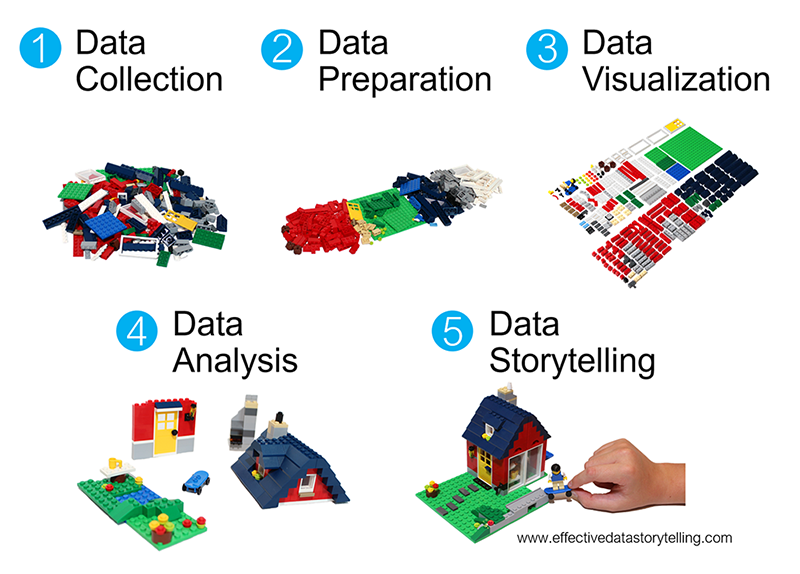
What’s coming up?

• In the last ~4-5 weeks we’ll focus on data storytelling through the completion of a course project.

• In the next ~1 week we’ll address the other gaps in the workflow: data collection and analysis. We’ll do so in the context of starting a data project…

Starting a data project

Any data science project consists of two phases:

1. data collection
   A data project starts with data! Thus far, you’ve either been given data, or used TidyTuesday data. In this unit:

   • We will explore how to find data, save data, import this data into RStudio, and do some preliminary data cleaning.
   • We won’t discuss how to collect data from scratch (e.g. via experiment, observational study, or survey).

2. data analysis
   Once we have data, we need to do some analysis. In this unit…

   • We will bring together our wrangling & visualization tools to discuss exploratory data analysis (EDA). EDA is the process of getting to know our data, obtaining insights from data, and using these insights to formulate, refine, and explore research questions.

   • We will not explore other types of analysis, such as modeling & prediction–if interested, take STAT 155 and 253 to learn more about these topics.

NOTE: These skills are best learned through practice. We’ll just scratch the surface here.

15.1 Warm-up

Before exploring how to find, store, import, check, and clean data, it’s important to recognize that data can be stored in various formats. We’ve been working with .csv files. In the background, these have “comma-separated values” (csv):

But there are many other common file types. For example, the following are compatible with R:

• Excel files: .xls, .xlsx
• R “data serialization” files: .rds
• files with tab-separated values: .tsv

STEP 1: Finding data files

Check Datasets for information about how to find a dataset that fits your needs.

STEP 2: Saving a local copy of the data file

Unless we’re just doing a quick, one-off data analysis, it’s important to store a local copy of a data file, i.e. save the data file to our own machine.

Mainly, we shouldn’t rely on another person / institution to store a data file online, in the same place, forever!

Saving Data

Saving your data…

• in a nice format (e.g. as a csv file)
• where you’ll be able to find it again
• ideally, within a folder that’s dedicated to the related project / assignment
• alongside the Rmd file(s) where you’ll record your analysis of the data

STEP 3: Importing the data file into RStudio

Once we have a local copy of our data file, we need to get it into RStudio! This process depends on 2 things: (1) the file type (e.g. .csv); and (2) the file location, i.e. where it’s stored on your computer.

1. FILE TYPE

The file type indicates which function we’ll need to import it. The table below lists some common import functions and when to use them.

Function	Data file type
read_csv()	.csv - you can save Excel files and Google Sheets as .csv
read_delim()	other delimited formats (tab, space, etc.)
read_sheet()	Google Sheet
st_read()	spatial data shapefile

NOTE: In comparison to read.csv, read_csv is faster when importing large data files and can more easily parse complicated datasets, eg, with dates, times, percentages.

2. FILE LOCATION

To import the data, we apply the appropriate function from above to the file path.

A file path is an address to where the file is stored on our computer or the web.

Consider “1600 Grand Ave, St. Paul, MN 55105”. Think about how different parts of the address give increasingly more specific information about the location. “St. Paul, MN 55105” tells us the city and smaller region within the city, “Grand Ave” tells us the street, and “1600” tells us the specific location on the street.

In the example below, the file path is absolute where it tells us the location giving more and more specific information as you read it from left to right.

• “~”, on an Apple computer, tells you that you are looking in the user’s home directory.
• “Desktop” tells you to go to the Desktop within that home directory.
• “112” tells you that you are looking in the 112 folder on the Desktop.
• “data” tells you to next go in the data folder in the 112 folder.
• “my_data.csv” tells you that you are looking for a file called my_data.csv location within the data folder.

library(tidyverse)
my_data <- read_csv("~/Desktop/112/data/my_data.csv")

STEP 4: Preliminary data checks and cleaning

Once the data is loaded, ask yourself a few questions:

What’s the structure of the data?

• Use str() to learn about the numbers of variables and observations as well as the classes or types of variables (date, location, string, factor, number, boolean, etc.)
• Use head() to view the top of the data table
• Use View() to view the data in a spreadsheet-like viewer

Is there anything goofy that we need to clean before we can analyze the data?

• Is it in a tidy format?
• How many rows are there? What does the row mean? What is an observation?
• Is there consistent formatting for categorical variables?
• Is there missing data that needs to be addressed?

STEP 5: Understanding the data

Start by understanding the data that is available to you. If you have a codebook, you have struck gold! If not (the more common case), you’ll need to do some detective work that often involves talking to people.

At this stage, ask yourself:

• Where does my data come from? How was it collected?¹
• Is there a codebook? If not, how can I learn more about it?
• Are there people I can reach out to who have experience with this data?

15.2 Exercises

Suppose our goal is to work with data on movie reviews, and that we’ve already gone through the work to find a dataset. The “imdb_5000_messy.csv” file is posted on Moodle. Let’s work with it!

Exercise 1: Save a local copy of the data file

Part a

On your laptop:

• Download the “imdb_5000_messy.csv” file from Moodle
• Move it to the data folder you created at the beginning of class

Part b

Hot tip: After saving your data file, it’s important to record appropriate citations and info in either a new Rmd (eg: “imdb_5000_messy_README.Rmd”) or in the Rmd where you’ll analyze the data. These citations should include:

• the data source, i.e. where you found the data
• the data creator, i.e. who / what group collected the original data
• possibly a data codebook, i.e. descriptions of the data variables

To this end, check out where we originally got our IMDB data:

https://www.kaggle.com/datasets/tmdb/tmdb-movie-metadata

After visiting that website, take some quick notes here on the data source and creator.

Exercise 2: Import the data into RStudio

Now that we have a local copy of our data file, let’s get it into RStudio! Remember that this process depends on 2 things: the file type and location. Since our file type is a csv, we can import it using read_csv(). But we have to supply the file location through a file path. To this end, we can either use an absolute file path or a relative file path.

Part a

An absolute file path describes the location of a file starting from the root or home directory. How we refer to the user root directory depends upon your machine:

• On a Mac: ~
• On Windows: typically C:\

Then the complete file path to the IMDB data file in the data folder, depending on your machine an where you created your portfolio project, can be:

• On a Mac: ~/Desktop/portfolio/data/imdb_5000_messy.csv
• On Windows: C:\Desktop\portfolio\data\imdb_5000_messy.csv or C:\\Desktop\\portfolio\\data\\imdb_5000_messy.csv

Putting this together, use read_csv() with the appropriate absolute file path to import your data into RStudio. Save this as imdb_messy.

library(tidyverse)
# imdb_messy <- read_csv("___")

Part b

Absolute file paths can get really long, depending upon our number of sub-folders, and they should not be used when sharing code with other and instead relative file paths should be used. A relative file path describes the location of a file from the current “working directory”, i.e. where RStudio would currently look for on your computer. Check what your working directory is inside this Rmd:

# This should be the folder where you stored this Rmd!
getwd()

[1] "/home/runner/work/mac-comp112website-f24/mac-comp112website-f24/activities"

Next, check what the working directory is for the console by typing getwd() in the console. This is probably different, meaning that the relative file paths that will work in your Rmd won’t work in the console! You can either exclusively work inside your Rmd, or change the working directory in your console, by navigating to the following in the upper toolbar: Session > Set Working Directory > To Source File location.

Part c

As is good practice, we created a data folder and saved our data file (imdb_5000_messy.csv) into.

Since our .Rmd analysis and .csv data live in the same project, we don’t have to write out absolute file paths that go all the way to the root directory. We can use relative file paths that start from where our code file exists to where the data file exist:

• On a Mac: ../data/imdb_5000_messy.csv
• On Windows: ..\data\imdb_5000_messy.csv or ..\\data\\imdb_5000_messy.csv

NOTE: .. means go one level up in the file hierarchy, ie, go to the parent folder/directory.

Putting this together, use read_csv() with the appropriate relative file path to import your data into RStudio. Save this as imdb_temp (temp for “temporary”). Convince yourself that this worked, i.e. you get the same dataset as imdb_messy.

#imdb_temp <- read_csv("___")

File Paths

Absolute file paths should be used when referring to files hosed on the web, eg, https://mac-stat.github.io/data/kiva_partners2.csv. In all other instances, relative file paths are recommended.

Part d: OPTIONAL

Sometimes, we don’t want to import the entire dataset. For example, we might want to…

• skips some rows (eg: if they’re just “filler”)
• only import the first “n” rows (eg: if the dataset is really large)
• only import a random subset of “n” rows (eg: if the dataset is really large)…

The “data import cheat sheet” at the top of this Rmd, or Google, are handy resources here. As one example…

Commenting/Uncommenting Code

To comment/uncomment several lines of code at once, highlight them then click ctrl/cmd+shift+c.

# Try importing only the first 5 rows
# read_csv("___", n_max = ___)

Exercise 3: Preliminary data checks

After importing new data into RStudio, you MUST do some quick checks of the data. Here are two first steps that are especially useful.

Part a

Open imdb_messy in the spreadsheet-like viewer by typing View(imdb_messy) in the console. Sort this “spreadsheet” by different variables by clicking on the arrows next to the variable names. Do you notice anything unexpected?

Part b

Do a quick summary() of each variable in the dataset. One way to do this is below:

# imdb_messy |>
#   mutate(across(where(is.character), as.factor)) |>  # convert characters to factors in order to summarize
#   summary()

Follow-up:

• What type of info is provided on quantitative variables?
• What type of info is provided on categorical variables?
• What stands out to you in these summaries? Is there anything you’d need to clean before using this data?

Exercise 4: Preliminary cleaning – factor variables 1

If you didn’t already in Exercise 3, check out the color variable in the imdb_messy dataset.

• What’s goofy about this / what do we need to fix?

• More specifically, what different categories does the color variable take, and how many movies fall into each of these categories?

Exercise 5: Preliminary cleaning – factor variables 2

When working with categorical variables like color, the categories must be “clean”, i.e. consistent and in the correct format. Let’s make that happen.

Part a

We could open the .csv file in, say, Excel or Google sheets, clean up the color variable, save a clean copy, and then reimport that into RStudio. BUT that would be the wrong thing to do. Why is it important to use R code, which we then save inside this Rmd, to clean our data?

Part b

Let’s use R code to change the color variable so that it appropriately combines the various categories into only 2: Color and Black_White. We’ve learned a couple sets of string-related tools that could be handy here. First, starting with the imdb_messy data, change the color variable using one of the functions we learned in Activity 12:

fct_relevel(), fct_recode(), fct_reorder()

Store your results in imdb_temp (don’t overwrite imdb_messy). To check your work, print out a count() table of the color variable in imdb_temp.

Part c

Repeat Part b using one of our string functions from the String chpater:

str_replace(), str_replace_all(), str_to_lower(), str_sub(), str_length(), str_detect()

Exercise 6: Preliminary cleaning – missing data 1

Throughout these exercises, you’ve probably noticed that there’s a bunch of missing data. This is encoded as NA (not available) in R. There are a few questions to address about missing data:

• How many values are missing data? What’s the volume of the missingness?
• Why are some values missing?
• What should we do about the missing values?

Let’s consider the first 2 questions in this exercise.

Part a

As a first step, let’s simply understand the volume of NAs. Specifically:

# Count the total number of rows in imdb_messy
#___(imdb_messy)

# Then count the number of NAs in each column
#colSums(is.na(imdb_messy))

# Then count the number of NAs in a specific column
#imdb_messy |> 
#  ___(___(is.na(actor_1_facebook_likes)))

Part b

As a second step, let’s think about why some values are missing. Study the individual observations with NAs carefully. Why do you think they are missing? Are certain films more likely to have more NAs than others?

Part c

Consider a more specific example. Obtain a dataset of movies that are missing data on actor_1_facebook_likes. Then explain why you think there are NAs. HINT: is.na(___)

Exercise 7: Preliminary cleaning – missing data 2

Next, let’s think about what to do about the missing values. There is no perfect or universal approach here. Rather, we must think carefully about…

• why the values are missing
• what we want to do with our data
• the impact of removing or replacing missing data on our work / conclusions

Part a

Calculate the average duration of a film. THINK: How can we deal with the NA’s?

Follow-up:

How are the NAs dealt with here? Did we have to create and save a new dataset in order to do this analysis?

Part b

Try out the drop_na() function:

# imdb_temp <- drop_na(imdb_messy)

Follow-up questions:

• What did drop_na() do? How many data points are left?
• In what situations might this function be a good idea?
• In what situations might this function be a bad idea?

Part c

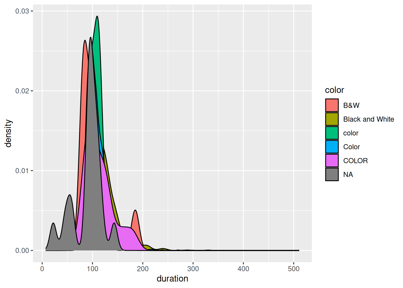
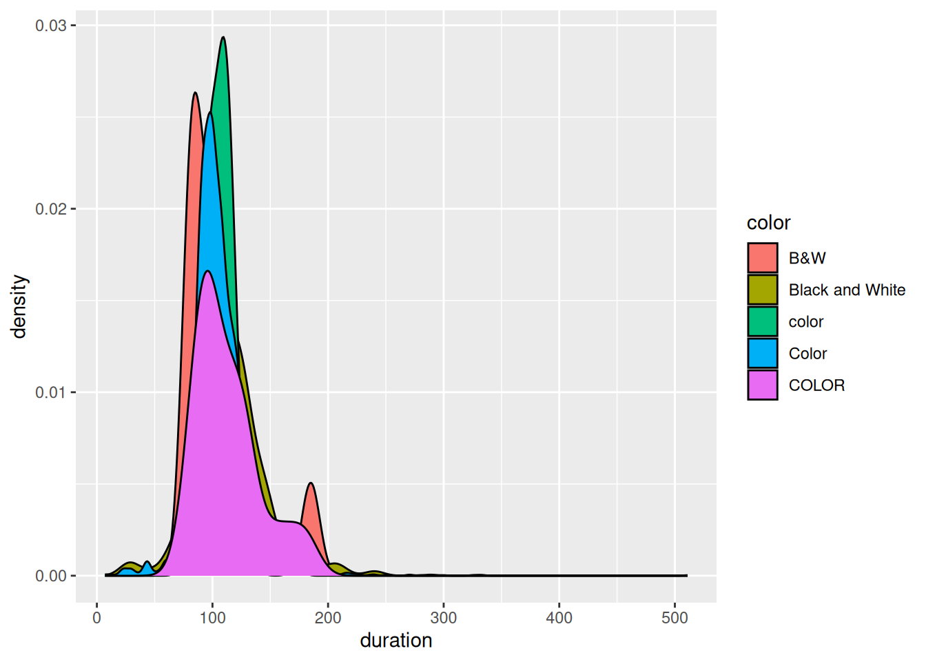
drop_na() removes data points that have any NA values, even if we don’t care about the variable(s) for which data is missing. This can result in losing a lot of data points that do have data on the variables we actually care about! For example, suppose we only want to explore the relationship between film duration and whether it’s in color. Check out a plot:

# ggplot(imdb_messy, aes(x = duration, fill = color)) + 
#   geom_density()

Follow-up:

• Create a new dataset with only and all movies that have complete info on duration and color. HINT: You could use !is.na(___) or drop_na() (differently than above)

• Use this new dataset to create a new and improved plot.

• How many movies remain in your new dataset? Hence why this is better than using the dataset from part b?

Part d

In some cases, missing data is more non-data than unknown data. For example, the films with NAs for actor_1_facebook_likes actually have 0 Facebook likes – they don’t even have actors! In these cases, we can replace the NAs with a 0. Use the replace_na() function to create a new dataset (imdb_temp) that replaces the NAs in actor_1_facebook_likes with 0. You’ll have to check out the help file for this function.

Exercise 8: New data + projects

Let’s practice the above ideas while also planting some seeds for the course project. Each group will pick and analyze their own dataset. The people you’re sitting with today aren’t necessarily your project groups! BUT do some brainstorming together:

• Share with each other: What are some personal hobbies or passions or things you’ve been thinking about or things you’d like to learn more about? Don’t think too hard about this! Just share what’s at the top of mind today.

• Each individual: Find a dataset online that’s related to one of the topics you shared in the above prompt.

• Discuss what data you found with your group!

• Load the data into RStudio, perform some basic checks, and perform some preliminary cleaning, as necessary.

15.3 Solutions

Click for Solutions

Exercise 3: Preliminary data checks

Part b

There are many NA’s, the color variable is goofy…

imdb_messy |>
  mutate(across(where(is.character), as.factor)) |>  # convert characters to factors in order to summarize
  summary()

      ...1                  color               director_name 
 Min.   :   1   B&W            :  10   Steven Spielberg:  26  
 1st Qu.:1262   Black and White: 199   Woody Allen     :  22  
 Median :2522   color          :  30   Clint Eastwood  :  20  
 Mean   :2522   Color          :4755   Martin Scorsese :  20  
 3rd Qu.:3782   COLOR          :  30   Ridley Scott    :  17  
 Max.   :5043   NA's           :  19   (Other)         :4834  
                                       NA's            : 104  
 num_critic_for_reviews    duration     director_facebook_likes
 Min.   :  1.0          Min.   :  7.0   Min.   :    0.0        
 1st Qu.: 50.0          1st Qu.: 93.0   1st Qu.:    7.0        
 Median :110.0          Median :103.0   Median :   49.0        
 Mean   :140.2          Mean   :107.2   Mean   :  686.5        
 3rd Qu.:195.0          3rd Qu.:118.0   3rd Qu.:  194.5        
 Max.   :813.0          Max.   :511.0   Max.   :23000.0        
 NA's   :50             NA's   :15      NA's   :104            
 actor_3_facebook_likes          actor_2_name  actor_1_facebook_likes
 Min.   :    0.0        Morgan Freeman :  20   Min.   :     0        
 1st Qu.:  133.0        Charlize Theron:  15   1st Qu.:   614        
 Median :  371.5        Brad Pitt      :  14   Median :   988        
 Mean   :  645.0        James Franco   :  11   Mean   :  6560        
 3rd Qu.:  636.0        Meryl Streep   :  11   3rd Qu.: 11000        
 Max.   :23000.0        (Other)        :4959   Max.   :640000        
 NA's   :23             NA's           :  13   NA's   :7             
     gross                            genres             actor_1_name 
 Min.   :      162   Drama               : 236   Robert De Niro:  49  
 1st Qu.:  5340988   Comedy              : 209   Johnny Depp   :  41  
 Median : 25517500   Comedy|Drama        : 191   Nicolas Cage  :  33  
 Mean   : 48468408   Comedy|Drama|Romance: 187   J.K. Simmons  :  31  
 3rd Qu.: 62309438   Comedy|Romance      : 158   Bruce Willis  :  30  
 Max.   :760505847   Drama|Romance       : 152   (Other)       :4852  
 NA's   :884         (Other)             :3910   NA's          :   7  
                    movie_title   num_voted_users   cast_total_facebook_likes
 Ben-Hur                  :   3   Min.   :      5   Min.   :     0           
 Halloween                :   3   1st Qu.:   8594   1st Qu.:  1411           
 Home                     :   3   Median :  34359   Median :  3090           
 King Kong                :   3   Mean   :  83668   Mean   :  9699           
 Pan                      :   3   3rd Qu.:  96309   3rd Qu.: 13756           
 The Fast and the Furious :   3   Max.   :1689764   Max.   :656730           
 (Other)                  :5025                                              
         actor_3_name  facenumber_in_poster
 Ben Mendelsohn:   8   Min.   : 0.000      
 John Heard    :   8   1st Qu.: 0.000      
 Steve Coogan  :   8   Median : 1.000      
 Anne Hathaway :   7   Mean   : 1.371      
 Jon Gries     :   7   3rd Qu.: 2.000      
 (Other)       :4982   Max.   :43.000      
 NA's          :  23   NA's   :13          
                                                                           plot_keywords 
 based on novel                                                                   :   4  
 1940s|child hero|fantasy world|orphan|reference to peter pan                     :   3  
 alien friendship|alien invasion|australia|flying car|mother daughter relationship:   3  
 animal name in title|ape abducts a woman|gorilla|island|king kong                :   3  
 assistant|experiment|frankenstein|medical student|scientist                      :   3  
 (Other)                                                                          :4874  
 NA's                                                                             : 153  
                                             movie_imdb_link
 http://www.imdb.com/title/tt0077651/?ref_=fn_tt_tt_1:   3  
 http://www.imdb.com/title/tt0232500/?ref_=fn_tt_tt_1:   3  
 http://www.imdb.com/title/tt0360717/?ref_=fn_tt_tt_1:   3  
 http://www.imdb.com/title/tt1976009/?ref_=fn_tt_tt_1:   3  
 http://www.imdb.com/title/tt2224026/?ref_=fn_tt_tt_1:   3  
 http://www.imdb.com/title/tt2638144/?ref_=fn_tt_tt_1:   3  
 (Other)                                             :5025  
 num_user_for_reviews     language       country       content_rating
 Min.   :   1.0       English :4704   USA    :3807   R        :2118  
 1st Qu.:  65.0       French  :  73   UK     : 448   PG-13    :1461  
 Median : 156.0       Spanish :  40   France : 154   PG       : 701  
 Mean   : 272.8       Hindi   :  28   Canada : 126   Not Rated: 116  
 3rd Qu.: 326.0       Mandarin:  26   Germany:  97   G        : 112  
 Max.   :5060.0       (Other) : 160   (Other): 406   (Other)  : 232  
 NA's   :21           NA's    :  12   NA's   :   5   NA's     : 303  
     budget            title_year   actor_2_facebook_likes   imdb_score   
 Min.   :2.180e+02   Min.   :1916   Min.   :     0         Min.   :1.600  
 1st Qu.:6.000e+06   1st Qu.:1999   1st Qu.:   281         1st Qu.:5.800  
 Median :2.000e+07   Median :2005   Median :   595         Median :6.600  
 Mean   :3.975e+07   Mean   :2002   Mean   :  1652         Mean   :6.442  
 3rd Qu.:4.500e+07   3rd Qu.:2011   3rd Qu.:   918         3rd Qu.:7.200  
 Max.   :1.222e+10   Max.   :2016   Max.   :137000         Max.   :9.500  
 NA's   :492         NA's   :108    NA's   :13                            
  aspect_ratio   movie_facebook_likes
 Min.   : 1.18   Min.   :     0      
 1st Qu.: 1.85   1st Qu.:     0      
 Median : 2.35   Median :   166      
 Mean   : 2.22   Mean   :  7526      
 3rd Qu.: 2.35   3rd Qu.:  3000      
 Max.   :16.00   Max.   :349000      
 NA's   :329                         

Exercise 4: Preliminary cleaning – factor variables 1

imdb_messy |> 
  count(color)

# A tibble: 6 × 2
  color               n
  <chr>           <int>
1 B&W                10
2 Black and White   199
3 COLOR              30
4 Color            4755
5 color              30
6 <NA>               19

Exercise 5: Preliminary cleaning – factor variables 2

Part a

That wouldn’t be reproducible. It’s important to log all steps in our data cleaning, so that we and others know and could reproduce those steps.

Part b

imdb_temp <- imdb_messy |> 
  mutate(color = fct_recode(color,
                            "Color" = "COLOR",
                            "Color" = "color",
                            "Black_White" = "B&W",
                            "Black_White" = "Black and White"))

imdb_temp |> 
  count(color)

# A tibble: 3 × 2
  color           n
  <fct>       <int>
1 Black_White   209
2 Color        4815
3 <NA>           19

Part c

imdb_temp <- imdb_messy |> 
  mutate(color = str_replace(color, "COLOR", "Color"),
         color = str_replace(color, "color", "Color"),
         color = str_replace(color, "B&W", "Black_White"),
         color = str_replace(color, "Black and White", "Black_White"))

imdb_temp |> 
  count(color)

# A tibble: 3 × 2
  color           n
  <chr>       <int>
1 Black_White   209
2 Color        4815
3 <NA>           19

Exercise 6: Preliminary cleaning – missing data 1

Part a

# Count the total number of rows in imdb_messy
nrow(imdb_messy)

[1] 5043

# Then count the number of NAs in each column
colSums(is.na(imdb_messy))

                     ...1                     color             director_name 
                        0                        19                       104 
   num_critic_for_reviews                  duration   director_facebook_likes 
                       50                        15                       104 
   actor_3_facebook_likes              actor_2_name    actor_1_facebook_likes 
                       23                        13                         7 
                    gross                    genres              actor_1_name 
                      884                         0                         7 
              movie_title           num_voted_users cast_total_facebook_likes 
                        0                         0                         0 
             actor_3_name      facenumber_in_poster             plot_keywords 
                       23                        13                       153 
          movie_imdb_link      num_user_for_reviews                  language 
                        0                        21                        12 
                  country            content_rating                    budget 
                        5                       303                       492 
               title_year    actor_2_facebook_likes                imdb_score 
                      108                        13                         0 
             aspect_ratio      movie_facebook_likes 
                      329                         0 

Part c

These are all documentaries that don’t have any actors.

imdb_messy |> 
  filter(is.na(actor_1_facebook_likes))

# A tibble: 7 × 29
   ...1 color director_name     num_critic_for_reviews duration
  <dbl> <chr> <chr>                              <dbl>    <dbl>
1  4503 Color Léa Pool                              23       97
2  4520 Color Harry Gantz                           12      105
3  4721 Color U. Roberto Romano                      3       80
4  4838 Color Pan Nalin                             15      102
5  4946 Color Amal Al-Agroobi                       NA       62
6  4947 Color Andrew Berends                        12       90
7  4991 Color Jem Cohen                             12      111
# ℹ 24 more variables: director_facebook_likes <dbl>,
#   actor_3_facebook_likes <dbl>, actor_2_name <chr>,
#   actor_1_facebook_likes <dbl>, gross <dbl>, genres <chr>,
#   actor_1_name <chr>, movie_title <chr>, num_voted_users <dbl>,
#   cast_total_facebook_likes <dbl>, actor_3_name <chr>,
#   facenumber_in_poster <dbl>, plot_keywords <chr>, movie_imdb_link <chr>,
#   num_user_for_reviews <dbl>, language <chr>, country <chr>, …

Exercise 7: Preliminary cleaning – missing data 2

Part a

imdb_messy |> 
  summarize(mean(duration, na.rm = TRUE))

# A tibble: 1 × 1
  `mean(duration, na.rm = TRUE)`
                           <dbl>
1                           107.

Follow-up:

We just remove the NAs from the calculation. No need to entirely remove the related movies from the dataset.

Part b

This gets rid of any movie with any NAs. There are only 3756 movies left! This approach is heavy-handed. It’s typically only a good idea when we need complete info on every variable for every part of our analysis.

imdb_temp <- drop_na(imdb_messy)
nrow(imdb_temp)

[1] 3756

colSums(is.na(imdb_temp))

                     ...1                     color             director_name 
                        0                         0                         0 
   num_critic_for_reviews                  duration   director_facebook_likes 
                        0                         0                         0 
   actor_3_facebook_likes              actor_2_name    actor_1_facebook_likes 
                        0                         0                         0 
                    gross                    genres              actor_1_name 
                        0                         0                         0 
              movie_title           num_voted_users cast_total_facebook_likes 
                        0                         0                         0 
             actor_3_name      facenumber_in_poster             plot_keywords 
                        0                         0                         0 
          movie_imdb_link      num_user_for_reviews                  language 
                        0                         0                         0 
                  country            content_rating                    budget 
                        0                         0                         0 
               title_year    actor_2_facebook_likes                imdb_score 
                        0                         0                         0 
             aspect_ratio      movie_facebook_likes 
                        0                         0 

Part c

ggplot(imdb_messy, aes(x = duration, fill = color)) +
  geom_density()

We keep most of the movies!

# Approach 1
imdb_temp <- imdb_messy |> 
  select(duration, color) |> 
  drop_na()
dim(imdb_temp)

[1] 5010    2

# Approach 2
imdb_temp <- imdb_messy |> 
  filter(!is.na(duration), !is.na(color))
dim(imdb_temp)

[1] 5010   29

# Plot
ggplot(imdb_temp, aes(x = duration, fill = color)) +
  geom_density()

Part d

imdb_temp <- imdb_messy |> 
  mutate(actor_1_facebook_likes =
         replace_na(actor_1_facebook_likes, 0))

imdb_temp |> 
  summarize(sum(is.na(actor_1_facebook_likes)))

# A tibble: 1 × 1
  `sum(is.na(actor_1_facebook_likes))`
                                 <int>
1                                    0

---

1. Particularly important questions about how it was collected include WHO (whether it is a sample of a larger data set, and, if so, how the sampling was done? Randomly? All cases during a specific time frame? All data for a selected set of users?), WHEN (is this current data or historical? what events may have had an impact?), WHAT (what variables were measured? how was it measured, self-reported through a questionnaire or measured directly?), WHY (who funded the data collection? for what purposes what the data collected? to whose benefit was the data collected?) Answers to such questions strongly impact the conclusions you will be able to draw from the data.