11  Joining Data

Learning Goals

Understand how to join different datasets:

• mutating joins: left_join(), inner_join() and full_join()
• filtering joins: semi_join(), anti_join()

Additional Resources

For more information about the topics covered in this chapter, refer to the resources below:

• Demonstration of joining data (YouTube) by Lisa Lendway
• Joings by Wickham, Çetinkaya-Rundel, & Grolemund
• Data wrangling on multiple tables by Baumer, Kaplan, and Horton

Instructions

General

• Be kind to yourself.
• Collaborate with and be kind to others. You are expected to work together as a group.
• Ask questions. Remember that we won’t discuss these exercises as a class.

Activity Specific

Help each other with the following:

• Create a new Quarto document in the activities folder of your portfolio project and do not forgot to include it in _quarto.yml file. Then click the </> Code link at the top right corner of this page and copy the code into the created Quarto document. This is where you’ll take notes. Remember that the portfolio is yours, so take notes in whatever way is best for you.
• Don’t start the Exercises section before we get there as a class. First, engage in class discussion and eventually collaborate with your group on the exercises!

11.1 Warm-up

Where are we? Data preparation

Thus far, we’ve learned how to:

• arrange() our data in a meaningful order
• subset the data to only filter() the rows and select() the columns of interest
• mutate() existing variables and define new variables
• summarize() various aspects of a variable, both overall and by group (group_by())
• reshape our data to fit the task at hand (pivot_longer(), pivot_wider())

Motivation

In practice, we often have to collect and combine data from various sources in order to address our research questions. Example:

• What are the best predictors of album sales?
  Combine:
  • Spotify data on individual songs (eg: popularity, genre, characteristics)
  • sales data on individual songs
• What are the best predictors of flight delays?
  Combine:
  • data on individual flights including airline, starting airport, and destination airport
  • data on different airlines (eg: ticket prices, reliability, etc)
  • data on different airports (eg: location, reliability, etc)

EXAMPLE 1

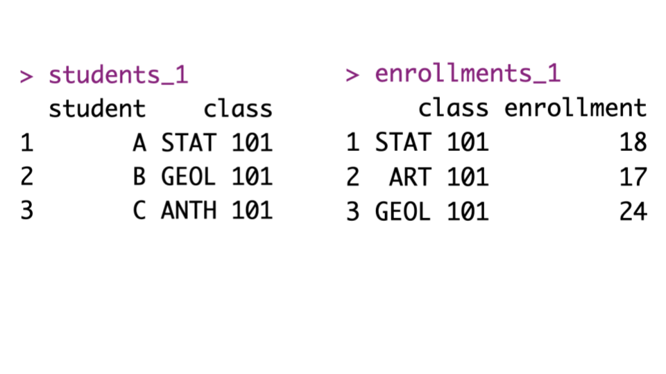
Consider the following (made up) data on students and course enrollments:

students_1 <- data.frame(
  student = c("A", "B", "C"),
  class = c("STAT 101", "GEOL 101", "ANTH 101")
)

# Check it out
students_1

  student    class
1       A STAT 101
2       B GEOL 101
3       C ANTH 101

enrollments_1 <- data.frame(
  class = c("STAT 101", "ART 101", "GEOL 101"),
  enrollment = c(18, 17, 24)
)

# Check it out
enrollments_1

     class enrollment
1 STAT 101         18
2  ART 101         17
3 GEOL 101         24

Our goal is to combine or join these datasets into one. For reference, here they are side by side:

First, consider the following:

• What variable or key do these datasets have in common? Thus by what information can we match the observations in these datasets?

• Relative to this key, what info does students_1 have that enrollments_1 doesn’t?

• Relative to this key, what info does enrollments_1 have that students_1 doesn’t?

EXAMPLE 2

There are various ways to join these datasets:

Let’s learn by doing. First, try the left_join() function:

library(tidyverse)
students_1 |> 
  left_join(enrollments_1)

  student    class enrollment
1       A STAT 101         18
2       B GEOL 101         24
3       C ANTH 101         NA

• What did this do? What are the roles of students_1 (the left table) and enrollments_1 (the right table)?

• What, if anything, would change if we reversed the order of the data tables? Think about it, then try.

EXAMPLE 3

Next, explore how our datasets are joined using inner_join():

students_1 |> 
  inner_join(enrollments_1)

  student    class enrollment
1       A STAT 101         18
2       B GEOL 101         24

• What did this do? What are the roles of students_1 (the left table) and enrollments_1 (the right table)?

• What, if anything, would change if we reversed the order of the data tables? Think about it, then try.

EXAMPLE 4

Next, explore how our datasets are joined using full_join():

students_1 |> 
  full_join(enrollments_1)

  student    class enrollment
1       A STAT 101         18
2       B GEOL 101         24
3       C ANTH 101         NA
4    <NA>  ART 101         17

• What did this do? What are the roles of students_1 (the left table) and enrollments_1 (the right table)?

• What, if anything, would change if we reversed the order of the data tables? Think about it, then try.

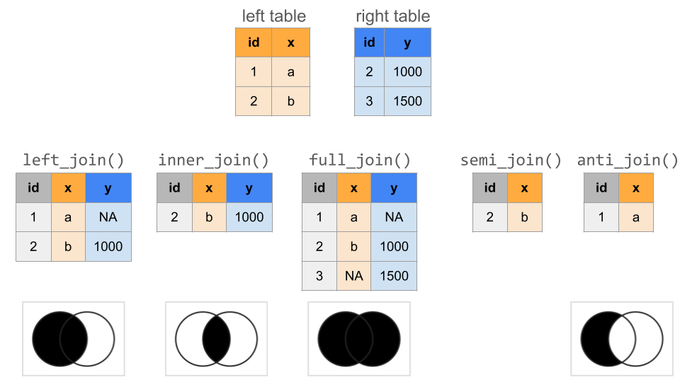
Mutating joins: left, inner, full

Mutating joins add new variables (columns) to the left data table from matching observations in the right table:

left_data |> mutating_join(right_data)

The most common mutating joins are:

• left_join()
  Keeps all observations from the left, but discards any observations in the right that do not have a match in the left.¹

• inner_join()
  Keeps only the observations from the left with a match in the right.

• full_join()
  Keeps all observations from the left and the right. (This is less common than left_join() and inner_join()).

NOTE: When an observation in the left table has multiple matches in the right table, these mutating joins produce a separate observation in the new table for each match.

EXAMPLE 5

Mutating joins combine information, thus increase the number of columns in a dataset (like mutate()). Filtering joins keep only certain observations in one dataset (like filter()), not based on rules related to any variables in the dataset, but on the observations that exist in another dataset. This is useful when we merely care about the membership or non-membership of an observation in the other dataset, not the raw data itself.

In our example data, suppose enrollments_1 only included courses being taught in the Theater building:

students_1 |> 
  semi_join(enrollments_1)

  student    class
1       A STAT 101
2       B GEOL 101

• What did this do? What info would it give us?

• How does semi_join() differ from inner_join()?

• What, if anything, would change if we reversed the order of the data tables? Think about it, then try.

EXAMPLE 6

Let’s try another filtering join for our example data:

students_1 |> 
  anti_join(enrollments_1)

  student    class
1       C ANTH 101

• What did this do? What info would it give us?

• What, if anything, would change if we reversed the order of the data tables? Think about it, then try.

Filtering joins: semi, anti

Filtering joins keep specific observations from the left table based on whether they match an observation in the right table.

• semi_join()
  Discards any observations in the left table that do not have a match in the right table. If there are multiple matches of right cases to a left case, it keeps just one copy of the left case.

• anti_join()
  Discards any observations in the left table that do have a match in the right table.

A SUMMARY OF ALL OF OUR JOINS

11.2 Exercises

Exercise 1: Where are my keys?

Part a

Define two new datasets, with different students and courses:

students_2 <- data.frame(
  student = c("D", "E", "F"),
  class = c("COMP 101", "BIOL 101", "POLI 101")
)

# Check it out
students_2

  student    class
1       D COMP 101
2       E BIOL 101
3       F POLI 101

enrollments_2 <- data.frame(
  course = c("ART 101", "BIOL 101", "COMP 101"),
  enrollment = c(18, 20, 19)
)

# Check it out
enrollments_2

    course enrollment
1  ART 101         18
2 BIOL 101         20
3 COMP 101         19

To connect the course enrollments to the students’ courses, try do a left_join(). You get an error! Identify the problem by reviewing the error message and the datasets we’re trying to join.

# eval = FALSE: don't evaluate this chunk when knitting. it produces an error.
students_2 |> 
  left_join(enrollments_2)

Part b

The problem is that course name, the key or variable that links these two datasets, is labeled differently: class in the students_2 data and course in the enrollments_2 data. Thus we have to specify these keys in our code:

students_2 |> 
  left_join(enrollments_2, by = c("class" = "course"))

  student    class enrollment
1       D COMP 101         19
2       E BIOL 101         20
3       F POLI 101         NA

# The order of the keys is important:
# by = c("left data key" = "right data key")
# The order is mixed up here, thus we get an error:
students_2 |> 
  left_join(enrollments_2, by = c("course" = "class"))

Part c

Define another set of fake data which adds grade information:

# Add student grades in each course
students_3 <- data.frame(
  student = c("Y", "Y", "Z", "Z"),
  class = c("COMP 101", "BIOL 101", "POLI 101", "COMP 101"),
  grade = c("B", "S", "C", "A")
)

# Check it out
students_3

  student    class grade
1       Y COMP 101     B
2       Y BIOL 101     S
3       Z POLI 101     C
4       Z COMP 101     A

# Add average grades in each course
enrollments_3 <- data.frame(
  class = c("ART 101", "BIOL 101","COMP 101"),
  grade = c("B", "A", "A-"),
  enrollment = c(20, 18, 19)
)

# Check it out
enrollments_3

     class grade enrollment
1  ART 101     B         20
2 BIOL 101     A         18
3 COMP 101    A-         19

Try doing a left_join() to link the students’ classes to their enrollment info. Did this work? Try and figure out the culprit by examining the output.

students_3 |> 
  left_join(enrollments_3)

  student    class grade enrollment
1       Y COMP 101     B         NA
2       Y BIOL 101     S         NA
3       Z POLI 101     C         NA
4       Z COMP 101     A         NA

Part d

The issue here is that our datasets have 2 column names in common: class and grade. BUT grade is measuring 2 different things here: individual student grades in students_3 and average student grades in enrollments_3. Thus it doesn’t make sense to try to join the datasets with respect to this variable. We can again solve this by specifying that we want to join the datasets using the class variable or key. What are grade.x and grade.y?

students_3 |> 
  left_join(enrollments_3, by = c("class" = "class"))

  student    class grade.x grade.y enrollment
1       Y COMP 101       B      A-         19
2       Y BIOL 101       S       A         18
3       Z POLI 101       C    <NA>         NA
4       Z COMP 101       A      A-         19

Exercise 2: More small practice

Before applying these ideas to bigger datasets, let’s practice identifying which join is appropriate in different scenarios. Define the following fake data on voters (people who have voted) and contact info for voting age adults (people who could vote):

# People who have voted
voters <- data.frame(
  id = c("A", "D", "E", "F", "G"),
  times_voted = c(2, 4, 17, 6, 20)
)

voters

  id times_voted
1  A           2
2  D           4
3  E          17
4  F           6
5  G          20

# Contact info for voting age adults
contact <- data.frame(
  name = c("A", "B", "C", "D"),
  address = c("summit", "grand", "snelling", "fairview"),
  age = c(24, 89, 43, 38)
)

contact

  name  address age
1    A   summit  24
2    B    grand  89
3    C snelling  43
4    D fairview  38

Use the appropriate join for each prompt below. In each case, think before you type:

• What dataset goes on the left?
• What do you want the resulting dataset to look like? How many rows and columns will it have?

# 1. We want contact info for people who HAVEN'T voted


# 2. We want contact info for people who HAVE voted


# 3. We want any data available on each person


# 4. When possible, we want to add contact info to the voting roster

Exercise 3: Bigger datasets

Let’s apply these ideas to some bigger datasets. In grades, each row is a student-class pair with information on:

• sid = student ID
• grade = student’s grade
• sessionID = an identifier of the class section

     sid grade   sessionID
1 S31185    D+ session1784
2 S31185    B+ session1785
3 S31185    A- session1791
4 S31185    B+ session1792
5 S31185    B- session1794
6 S31185    C+ session1795

In courses, each row corresponds to a class section with information on:

• sessionID = an identifier of the class section
• dept = department
• level = course level (eg: 100)
• sem = semester
• enroll = enrollment (number of students)
• iid = instructor ID

    sessionID dept level    sem enroll     iid
1 session1784    M   100 FA1991     22 inst265
2 session1785    k   100 FA1991     52 inst458
3 session1791    J   100 FA1993     22 inst223
4 session1792    J   300 FA1993     20 inst235
5 session1794    J   200 FA1993     22 inst234
6 session1795    J   200 SP1994     26 inst230

Use R code to take a quick glance at the data.

# How many observations (rows) and variables (columns) are there in the grades data?


# How many observations (rows) and variables (columns) are there in the courses data?

Exercise 4: Class size

How big are the classes?

Part a

Before digging in, note that some courses are listed twice in the courses data:

courses |> 
  count(sessionID) |> 
  filter(n > 1)

     sessionID n
1  session2047 2
2  session2067 2
3  session2448 2
4  session2509 2
5  session2541 2
6  session2824 2
7  session2826 2
8  session2862 2
9  session2897 2
10 session3046 2
11 session3057 2
12 session3123 2
13 session3243 2
14 session3257 2
15 session3387 2
16 session3400 2
17 session3414 2
18 session3430 2
19 session3489 2
20 session3524 2
21 session3629 2
22 session3643 2
23 session3821 2

If we pick out just 1 of these, we learn that some courses are cross-listed in multiple departments:

courses |> 
  filter(sessionID == "session2047")

For our class size exploration, obtain the total enrollments in each sessionID, combining any cross-listed sections. Save this as courses_combined. NOTE: There’s no joining to do here!

# courses_combined <- courses |> 
#   ___(sessionID) |> 
#   ___(enroll = sum(___))

# Check that this has 1695 rows and 2 columns
# dim(courses_combined)

Part b

Let’s first examine the question of class size from the administration’s viewpoint. To this end, calculate the median class size across all class sections. (The median is the middle or 50th percentile. Unlike the mean, it’s not skewed by outliers.) THINK FIRST:

• Which of the 2 datasets do you need to answer this question? One? Both?
• If you need course information, use courses_combined not courses.
• Do you have to do any joining? If so, which dataset will go on the left, i.e. which dataset includes your primary observations of interest? Which join function will you need?

Part c

But how big are classes from the student perspective? To this end, calculate the median class size for each individual student. Once you have the correct output, store it as student_class_size. THINK FIRST:

• Which of the 2 datasets do you need to answer this question? One? Both?
• If you need course information, use courses_combined not courses.
• Do you have to do any joining? If so, which dataset will go on the left, i.e. which dataset includes your primary observations of interest? Which join function will you need?

Part d

The median class size varies from student to student. To get a sense for the typical student experience and range in student experiences, construct and discuss a histogram of the median class sizes experienced by the students.

# ggplot(student_class_size, aes(x = ___)) + 
#   geom___()

Exercise 5: Narrowing in on classes

Part a

Show data on the students that enrolled in session1986. THINK FIRST: Which of the 2 datasets do you need to answer this question? One? Both?

Part b

Below is a dataset with all courses in department E:

dept_E <- courses |> 
  filter(dept == "E")

What students enrolled in classes in department E? (We just want info on the students, not the classes.)

Exercise 6: All the wrangling

Use all of your wrangling skills to answer the following prompts! THINK FIRST:

• Think about what tables you might need to join (if any). Identify the corresponding variables to match.
• You’ll need an extra table to convert grades to grade point averages:

gpa_conversion <- tibble(
  grade = c("A+", "A", "A-", "B+", "B", "B-", "C+", "C", "C-", "D+", "D", "D-", "NC", "AU", "S"), 
  gp = c(4.3, 4, 3.7, 3.3, 3, 2.7, 2.3, 2, 1.7, 1.3, 1, 0.7, 0, NA, NA)
)

gpa_conversion

# A tibble: 15 × 2
   grade    gp
   <chr> <dbl>
 1 A+      4.3
 2 A       4  
 3 A-      3.7
 4 B+      3.3
 5 B       3  
 6 B-      2.7
 7 C+      2.3
 8 C       2  
 9 C-      1.7
10 D+      1.3
11 D       1  
12 D-      0.7
13 NC      0  
14 AU     NA  
15 S      NA  

Part a

How many total student enrollments are there in each department? Order from high to low.

Part b

What’s the grade-point average (GPA) for each student?

Part c

What’s the median GPA across all students?

Part d

What fraction of grades are below B+?

Part e

What’s the grade-point average for each instructor? Order from low to high.

Part f

CHALLENGE: Estimate the grade-point average for each department, and sort from low to high. NOTE: Don’t include cross-listed courses. Students in cross-listed courses could be enrolled under either department, and we do not know which department to assign the grade to. HINT: You’ll need to do multiple joins.

Exercise 7: HOMEWORK PRACTICE

This exercise is on Homework 4, thus no solutions are provided. In Homework 4, you’ll be working with the Birthdays data:

library(mosaic)
data("Birthdays")
head(Birthdays)

  state year month day       date wday births
1    AK 1969     1   1 1969-01-01  Wed     14
2    AL 1969     1   1 1969-01-01  Wed    174
3    AR 1969     1   1 1969-01-01  Wed     78
4    AZ 1969     1   1 1969-01-01  Wed     84
5    CA 1969     1   1 1969-01-01  Wed    824
6    CO 1969     1   1 1969-01-01  Wed    100

You’ll also be exploring how the number of daily births is (or isn’t!) related to holidays. To this end, import data on U.S. federal holidays here. NOTE: lubridate::dmy() converts the character-string date stored in the CSV to a “POSIX” date-number.

holidays <- read.csv("https://mac-stat.github.io/data/US-Holidays.csv") |>
  mutate(date = as.POSIXct(lubridate::dmy(date)))

Part a

Create a new dataset, daily_births_1980, which:

• keeps only daily_births related to 1980
• adds a variable called is_holiday which is TRUE when the day is a holiday, and FALSE otherwise. NOTE: !is.na(x) is TRUE if column x is not NA, and FALSE if it is NA.

Print out the first 6 rows and confirm that your dataset has 366 rows (1 per day in 1980) and 7 columns. HINT: You’ll need to combine 2 different datasets.

# Define daily_births_1980


# Check out the first 6 rows


# Confirm that daily_births_1980 has 366 rows and 7 columns

Part b

Plot the total number of babies born (y-axis) per day (x-axis) in 1980. Color each date according to its day of the week, and shape each date according to whether or not it’s a holiday. (This is a modified version of 3c!)

Part c

Discuss your observations. For example: To what degree does the theory that there tend to be fewer births on holidays hold up? What holidays stand out the most?

Part d (OPTIONAL)

Some holidays stand out more than others. It would be helpful to label them. Use geom_text to add labels to each of the holidays. NOTE: You can set the orientation of a label with the angle argument; e.g., geom_text(angle = 40, ...).

Next steps

If you finish this all during class, you’re expected to work on Homework 4. If you’re done with Homework 4, you’re expected to play around with more TidyTuesday data. Mainly, and naturally, you’re expected to spend 112 class time on 112 :)

11.3 Solutions

Click for Solutions

EXAMPLE 1

1. class
2. a student that took ANTH 101
3. data on ART 101

EXAMPLE 2

• What did this do? Linked course info to all students in students_1
• Which observations from students_1 (the left table) were retained? All of them.
• Which observations from enrollments_1 (the right table) were retained? Only STAT and GEOL, those that matched the students.
• What, if anything, would change if we reversed the order of the data tables? Think about it, then try. We retain the courses, not students.

enrollments_1 |> 
  left_join(students_1)

     class enrollment student
1 STAT 101         18       A
2  ART 101         17    <NA>
3 GEOL 101         24       B

EXAMPLE 3

• Which observations from students_1 (the left table) were retained? A and B, only those with enrollment info.

• Which observations from enrollments_1 (the right table) were retained? STAT and GEOL, only those with studen info.

• What, if anything, would change if we reversed the order of the data tables? Think about it, then try. Same info, different column order.

enrollments_1 |> 
    inner_join(students_1)

     class enrollment student
1 STAT 101         18       A
2 GEOL 101         24       B

EXAMPLE 4

• Which observations from students_1 (the left table) were retained? All
• Which observations from enrollments_1 (the right table) were retained? All
• What, if anything, would change if we reversed the order of the data tables? Think about it, then try. Same data, different order.

enrollments_1 |> 
    full_join(students_1)

     class enrollment student
1 STAT 101         18       A
2  ART 101         17    <NA>
3 GEOL 101         24       B
4 ANTH 101         NA       C

EXAMPLE 5

• Which observations from students_1 (the left table) were retained? Only those with enrollment info.
• Which observations from enrollments_1 (the right table) were retained? None.
• What, if anything, would change if we reversed the order of the data tables? Think about it, then try. Same data, different order.

enrollments_1 |> 
  semi_join(students_1)

     class enrollment
1 STAT 101         18
2 GEOL 101         24

EXAMPLE 6

• Which observations from students_1 (the left table) were retained? Only C, the one without enrollment info.
• Which observations from enrollments_1 (the right table) were retained? None.
• What, if anything, would change if we reversed the order of the data tables? Think about it, then try. Retain only ART 101, the course with no student info.

enrollments_1 |> 
  anti_join(students_1)

    class enrollment
1 ART 101         17

Exercise 2: More small practice

# 1. We want contact info for people who HAVEN'T voted
contact |> 
  anti_join(voters, by = c("name" = "id"))

  name  address age
1    B    grand  89
2    C snelling  43

# 2. We want contact info for people who HAVE voted
contact |> 
  semi_join(voters, by = c("name" = "id"))

  name  address age
1    A   summit  24
2    D fairview  38

# 3. We want any data available on each person
contact |> 
  full_join(voters, by = c("name" = "id"))

  name  address age times_voted
1    A   summit  24           2
2    B    grand  89          NA
3    C snelling  43          NA
4    D fairview  38           4
5    E     <NA>  NA          17
6    F     <NA>  NA           6
7    G     <NA>  NA          20

voters |> 
  full_join(contact, by = c("id" = "name"))

  id times_voted  address age
1  A           2   summit  24
2  D           4 fairview  38
3  E          17     <NA>  NA
4  F           6     <NA>  NA
5  G          20     <NA>  NA
6  B          NA    grand  89
7  C          NA snelling  43

# 4. We want to add contact info, when possible, to the voting roster
voters |> 
  left_join(contact, by = c("id" = "name"))

  id times_voted  address age
1  A           2   summit  24
2  D           4 fairview  38
3  E          17     <NA>  NA
4  F           6     <NA>  NA
5  G          20     <NA>  NA

Exercise 3: Bigger datasets

# How many observations (rows) and variables (columns) are there in the grades data?
dim(grades)

[1] 5844    3

# How many observations (rows) and variables (columns) are there in the courses data?
dim(courses)

[1] 1718    6

Exercise 4: Class size

Part a

courses_combined <- courses |>
  group_by(sessionID) |>
  summarize(enroll = sum(enroll))

# Check that this has 1695 rows and 2 columns
dim(courses_combined)

[1] 1695    2

Part b

courses_combined |> 
  summarize(median(enroll))

Part c

student_class_size <- grades |> 
  left_join(courses_combined) |> 
  group_by(sid) |> 
  summarize(med_class = median(enroll))

head(student_class_size)

Part d

ggplot(student_class_size, aes(x = med_class)) +
  geom_histogram(color = "white")

Exercise 5: Narrowing in on classes

Part a

grades |> 
  filter(sessionID == "session1986")

Part b

grades |> 
  semi_join(dept_E)

Exercise 6: All the wrangling

Part a

courses |> 
  group_by(dept) |> 
  summarize(total = sum(enroll)) |> 
  arrange(desc(total))

Part b

grades |> 
  left_join(gpa_conversion) |> 
  group_by(sid) |> 
  summarize(mean(gp, na.rm = TRUE))

Part c

grades |> 
  left_join(gpa_conversion) |> 
  group_by(sid) |> 
  summarize(gpa = mean(gp, na.rm = TRUE)) |> 
  summarize(median(gpa))

Part d

# There are lots of approaches here!
grades |> 
  left_join(gpa_conversion) |> 
  mutate(below_b_plus = (gp < 3.3)) |> 
  summarize(mean(below_b_plus, na.rm = TRUE))

Part e

grades |> 
  left_join(gpa_conversion) |> 
  left_join(courses) |> 
  group_by(iid) |> 
  summarize(gpa = mean(gp, na.rm = TRUE)) |> 
  arrange(gpa)

Part f

cross_listed <- courses |> 
  count(sessionID) |> 
  filter(n > 1)

grades |> 
  anti_join(cross_listed) |> 
  inner_join(courses) |> 
  left_join(gpa_conversion) |> 
  group_by(dept) |> 
  summarize(gpa = mean(gp, na.rm = TRUE)) |> 
  arrange(gpa)

---

1. There is also a right_join() that adds variables in the reverse direction from the left table to the right table, but we do not really need it as we can always switch the roles of the two tables.︎